Solver Max - Optimal rational approximation using SciPy

7 January 2025

https://en.wikipedia.org/wiki/Aryabhata

In this article we solve a non-linear curve fitting problem using the SciPy library. SciPy is especially well-suiting to solving this type of problem, as it includes a variety of functions for fitting and optimizing non-linear functions.

Along the way, we illustrate how to use SciPy's curve_fit and minimize functions for this type of task. In addition, we look at some good practices to apply when solving this type of problem, including:

Using different criteria for defining the best fit, such as sum of squared differences and largest absolute error.
Examining use of the full_output option when using the curve_fit function, to get more information about the result.
Examining the success and message values of the minimize function result to ensure that the solver converges correctly.
Trying a variety of minimize solution methods to see which one works best in our specific situation.
Fine-tuning the solution by changing the convergence tolerance.

Download the models

The models described in this article are built in Python, using the SciPy library.

The files are available on GitHub.

Situation

John Cook has a series of blog posts about approximating trigonometric functions using ratios of quadratic polynomials. We choose one example as the basis for our non-linear curve fitting task. That is, the following approximation of the cosine function is attributed to the mathematician-astronomer Aryabhata (476–550 CE):

\begin{alignat*}{1} &\text{cos } x \approx \frac{\pi^2 - 4x^2}{\pi^2 + x^2}\\ \end{alignat*}

A more general form of this function is:

\begin{alignat*}{1} &\text{cos } x \approx \frac{\text{a} + \text{b}x^2}{\text{c} + \text{d}x^2}, \quad \text{where } -\frac{\pi}{2} \le x \le +\frac{\pi}{2}\\ \end{alignat*}

Our goal is to find optimal values for the coefficients \(\text{a}\), \(\text{b}\), \(\text{c}\), and \(\text{d}\) to minimize the difference between the cosine function and the approximation function. This is a type of curve-fitting problem.

Model 1: Curve fitting

An obvious way to solve the problem is to use SciPy's curve_fit function. Part of our code for implementing this approach is shown in Figure 1.

Figure 1. Part of Model 1's code

def model(x, b, c, d):
    return (A + b * x**2) / (c + d * x**2)

def target_function(x):
    return np.cos(x)

def main():
    print('SciPy curve_fit')
    print('===============\n')
    x_data = np.linspace(-np.pi/2, np.pi/2, NUMPOINTS)
    y_data = target_function(x_data)
    guess = [1, 1, 1]
    result, pcov, infodict, mesg, ier = curve_fit(model, x_data, y_data, p0=guess, full_output=True)
    difference = y_data - model(x_data, *result)
    print_results(result, x_data, y_data, mesg, ier, difference)
    plot_results(result, x_data, y_data, difference)

NUMPOINTS = 10000
A = np.pi**2

Consistent with Dr. Cook's approach, we set the value of one coefficient as a constant and optimize over the remaining coefficients. That is, we set A = np.pi**2 (9.86960440).

We call SciPy's curve_fit function. The fit is evaluated over a set of \(x\) and \(y\) pairs – we specify 10,000 points, which should be more than enough to get a good representation of the functions. We also specify an initial guess for the three unknown coefficients \(\text{b}\), \(\text{c}\), and \(\text{d}\). The accuracy of the initial guess isn't especially important for this model, provided it isn't wildly wrong, but for some models it may be critical.

Finally, we specify the option full_output. When True, this option prompts the curve_fit function to return additional information that helps us understand the solution. It is a good practice to always look at this additional information, to ensure that the fitting process works as expected.

The output from running Model 1 is shown in Figure 2. SciPy's status and message indicate that the fitting process succeeded. The optimal parameters are very close to Aryabhata's values of \(+\pi^2\), -4, \(+\pi^2\), and +1. We also print the sum of squared differences between the target and fitted function, plus the maximum and minimum differences between the functions – all of which are small, indicating that the model is a very good fit.

Figure 2. Model 1's output

Status:  True
Message: Both actual and predicted relative reductions in the sum of squares are at most 0.000000
         and the relative error between two consecutive iterates is at most 0.000000

Fitted parameters:
a   =   9.86960440
b   =  -4.01047621
c   =   9.86327195
d   =   0.98120671

Sum squared diffs: 0.003446

Difference extremes:
Max =   0.00210423
Min =  -0.00086865

Figure 3 plots the target cosine function and fitted model function, along with the differences between the two functions. Here we can see that the fit is good, with very small differences between the functions.

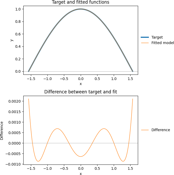
Model 1 plots — Figure 3. Model 1's plots

But there's a problem: Our result does not match the solution found by Dr. Cook. It is close, but materially different.

The issue is that the curve_fit function minimizes the sum of squared differences between the functions, while Dr. Cook is minimizing the largest absolute error. So, we need to take a different approach.

Model 2: Minimize sum of squared differences

We can use SciPy's minimize function to find optimal values for the coefficients given our non-linear target and model functions. As a test, we first look to minimize the sum of squared differences between the functions, like we did in Model 1. Later, we'll change that to minimize the largest absolute error.

Figure 4 shows part of Model 2's code. The main differences from Model 1 are that we introduce an objective function and call minimize rather than curve_fit. The objective function is defined as the sum of squared differences between the functions.

A frustrating feature of the SciPy is that there are inconsistencies between how various functions are used. In this case, when calling the minimize function we need to use result.x rather than the result object we use with the curve_fit function. Note that the result is always called x, unrelated to how we defined our data (which happens to be called x and y).

Figure 4. Part of Model 2's code

def objective(guess, x, y):
    b, c, d = guess
    return np.sum((y - model(x, b, c, d))**2)

def main():
    print('SciPy optimize (minimize sum of squared differences)')
    print('====================================================\n')
    x_data = np.linspace(-np.pi/2, np.pi/2, NUMPOINTS)
    y_data = target_function(x_data)
    guess = [1, 1, 1]
    result = minimize(objective, guess, args=(x_data, y_data))
    difference = y_data - model(x_data, *result.x)
    print_results(result, x_data, y_data, difference)
    plot_results(result.x, x_data, y_data, difference)

The result for Model 2 is identical to Model 1. This is reassuring, as it indicates that we've implemented Model 2 correctly.

Model 3: Minimize largest absolute error

Now we can modify Model 2 to minimize the largest absolute error. All we need to do to make Model 3 is to change the objective function, as shown in Figure 5. This objective function minimizes the maximum absolute difference between the target and fitted functions.

Note that SciPy is very versatile is the variety of math functions that it can evaluate. In this case, we use the max and abs functions directly in the objective function – which we could not do in, for example, a Pyomo model.

Figure 5. Part of Model 3's code

def objective(guess, x, y):
    b, c, d = guess
    return np.max(np.abs(y - model(x, b, c, d)))

The output from Model 3 is shown in Figure 6. The sum of squared differences (80.436383) is several orders of magnitude worse than the result from Models 1 and 2 (0.003446). Also, SciPy's status and message tell us that the model did not converge properly.

Note that when using the minimize function, we get these results directly from the result object as result.success and result.message – another inconsistency between the minimize and curve_fit functions.

Figure 6. Model 3's output

Status:  False
Message: Desired error not necessarily achieved due to precision loss.

Fitted parameters:
a   =   9.86960440
b   =  -2.35427921
c   =   9.20083645
d   =   9.11915102

Sum squared diffs: 80.436383

Difference extremes:
Max =   0.14267529
Min =  -0.12809050

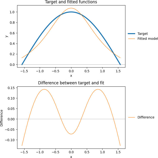
Looking at the plots of the fit and differences, shown in Figure 7, we see that the modelled function is clearly not a good fit. Note that the vertical axis scale in the difference plot of Figure 7 is 100 times larger than the equivalent scale for Model 1 in Figure 3. Obviously, this is nowhere near as good a fit as that achieved with Models 1 and 2.

Model 3 plots — Figure 7. Model 3's plots

Model 4: Try a variety of multivariate optimization methods

A problem with Model 3 is that we didn't specify the method that SciPy should use to perform the minimization. SciPy has more than a dozen methods available to the minimize function when performing multivariate optimization.

By omitting the method, we rely on SciPy to choose a default method (in this case it chose the BFGS method). Using the default is generally a bad idea. Better practice is to explicitly specify the method.

Choosing an appropriate optimization method is a tricky business. There is some advice available in the article Choosing a method. But often the best way to choose a method is to try a few and see which one works best.

So, that's exactly what we do in Model 4. As shown in Figure 8, we loop over the minimization process using a selection of different methods, collating the results for each. We've chosen the methods that don't need a Hessian or Jacobian matrix to be specified, as our objective function of minimizing the maximum absolute difference isn't differentiable.

Figure 8. Part of Model 4's code

def main():
    print('SciPy optimize (minimize maximum absolute difference, various methods)')
    print('======================================================================\n')
    x_data = np.linspace(-np.pi/2, np.pi/2, NUMPOINTS)
    y_data = target_function(x_data)
    guess = [1, 1, 1]
    methods = ['Nelder-Mead', 'Powell', 'CG', 'BFGS', 'L-BFGS-B', 'TNC', 'COBYLA', 'SLSQP']
    
    results = []
    for method in methods:
        result = minimize(objective, guess, args=(x_data, y_data), method=method)
        difference = y_data - model(x_data, *result.x)
        success = result.success
        message = result.message
        results.append([method, result.x, difference, success, message])
    
    print_results(results, x_data, y_data, difference)
    plot_results(results, x_data, y_data)

The output from running Model 4 is shown in Figure 9. Not all the methods report success, and only one method (Nelder-Mead) finds a good solution.

Figure 9. Model 4's output

Method          SS Diff    Max diff    Min diff    Success    Message                                 
---------------------------------------------------------------------------------------------------------------------------
Nelder-Mead    0.004676    0.000973   -0.000970    True       Optimization terminated successfully.   
Powell        42.836108    0.096857   -0.096857    True       Optimization terminated successfully.   
CG            55.307308    0.107355   -0.107355    False      Desired error not necessarily achieved due to precision loss.
BFGS          80.436383    0.142675   -0.128091    False      Desired error not necessarily achieved due to precision loss.
L-BFGS-B      17.010731    0.064772   -0.064772    True       CONVERGENCE: REL_REDUCTION_OF_F_<=_FACTR*EPSMCH
TNC           59.293782    0.112022   -0.112021    True       Converged (|f_n-f_(n-1)| ~= 0)          
COBYLA        26.658194    0.082261   -0.082248    True       Optimization terminated successfully.   
SLSQP          3.033454    0.027041   -0.027041    True       Optimization terminated successfully

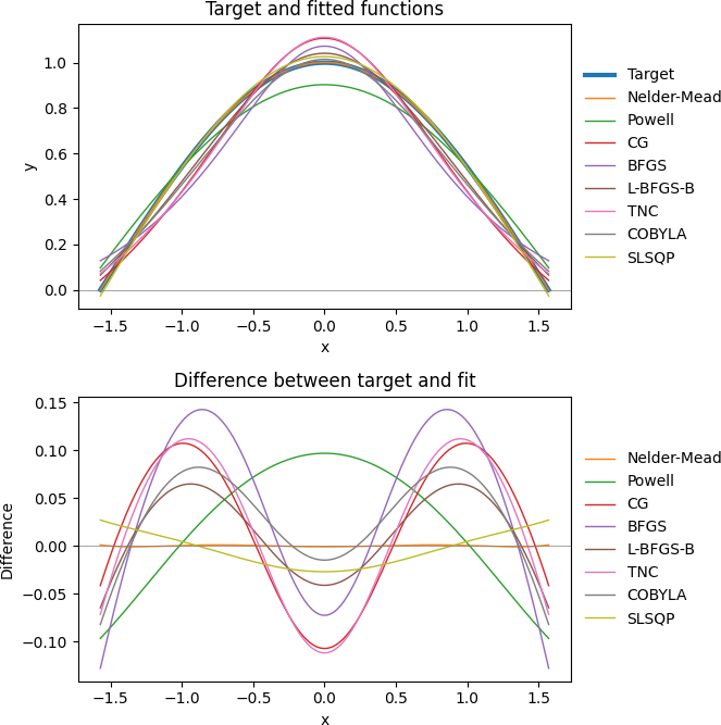
Figure 10 plots the target cosine function and model functions, along with the differences between the functions. Here we can see that the various methods produce a variety of fits. Relative to the other methods, the Nelder-Mead method's differences are very close to zero – which is what we want. Importantly, the results for the Nelder-Mead method are very similar to the results described in Dr. Cook's blog.

Model 4 plots — Figure 10. Model 4's plots

Model 5: Minimize largest absolute error using the Nelder-Mead method

Having identified a good method for our model, we can make one more refinement. Dr. Cook mentions that the pattern of differences should be symmetrical, with the maximum and minimum differences having the same absolute values. In Model 4, our difference extremes are Max = 0.000973 and Min = -0.000970. These are very close to being the same, but not quite. In practical terms, the difference between the extremes likely doesn't matter, but let's try to tighten the solution anyway.

Another option we can apply to the minimize function is a convergence tolerance. We modify Model 3 to produce Model 5 by changing just the one line shown in Figure 11. That is, we specify method='Nelder-Mead' and the convergence tolerance tol=1e-9. For the tolerance, we use a very small number, to ensure that the solution is nicely symmetrical.

Figure 11. Part of Model 5's code

result = minimize(objective, guess, args=(x_data, y_data), method='Nelder-Mead', tol=1e-9)

The result is shown in Figure 12. The absolute value of the difference max and min extremes are identical (to 8 decimal places), as intended.

Note that the sum of squared differences for Model 5 of 0.004668 is slightly worse than the result for Model 1 of 0.003446. This is due to Model 5 minimizing the maximum absolute difference (extreme points) rather than minimizing the sum of squared differences (over all points).

Figure 12. Model 5's output

Status:  True
Message: Optimization terminated successfully.

Fitted parameters:
a   =   9.86960440
b   =  -4.00484833
c   =   9.86004032
d   =   1.00226119

Sum squared diffs: 0.004668

Difference extremes:
Max =   0.00096998
Min =  -0.00096998

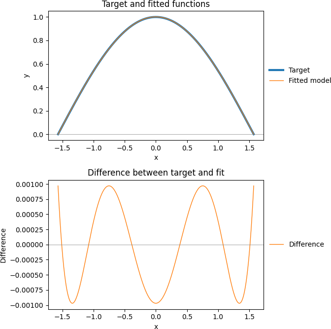
Looking at the plot of the differences, shown in Figure 13, we see that the seven extreme points all look to have about the same absolute value. Examining the data in more detail, we confirm that all seven extreme points have the value +0.00096998 or -0.00096998. This complies with the "Equioscillation characterization of best approximants" theorem described by Dr. Cook. Therefore, we have achieved our goal of optimally approximating a trigonometric function using ratios of quadratic polynomials.

Model 5 plots — Figure 13. Model 5's plots

Conclusion

In this article, we find the optimal rational approximation of a trigonometric function using ratios of quadratic polynomials.

Our models illustrate the use of SciPy's curve_fit and minimize functions for multivariate data. We also apply some good practices in our modelling, specifically:

Specify the full_output option when using the curve_fit function, to get more information about the result.
Examine the success and message values of the minimize function result to ensure that the solver converges correctly.
When solving non-linear functions, try a variety of solution methods to see which one works best in your specific situation.
Consider changing the convergence tolerance, to fine-tune the solution.

If you would like to know more about this model, or you want help with your own models, then please contact us.