Solver Max - Objectives matter: Sorting using a MIP model

14 November 2024

We replicate a model by Erwin Kalvelagen at Yet Another Math Programming Consultant (YAMPC), Sorting using a MIP model. Erwin explores the run time behaviour of the CPLEX, HiGHS, and Xpress solvers for this feasibility problem, using an objective function that has a constant value of zero.

Professor Paul Rubin explores the same model in Solver parameters matter, using the CPLEX and Xpress solvers, finding that small tweaks to the solver options can have large impacts on relative solver performance.

In this article, we assess the impact of using an alternative objective function in the same model. The idea is to give the HiGHS solver greater traction while working through the solution space, hopefully helping it to solve the model faster. We've found this technique to be useful for some other models – will it help in this situation?

Download the models

The model described in this article is built in Python, using the Pyomo library.

The files are available on GitHub.

Situation

The situation is very simple:

Input: a 1-dimensional parameter with values.
Output: a 1-dimensional variable with the values sorted in ascending order.

Sorting a parameter within a Mixed Integer Linear Program can be solved as a feasibility problem. That is, we don't need an objective function. Instead, we just want to find a feasible solution. Finding a feasible solution is a fairly common modelling requirement, though in this situation the solution is unique (assuming no duplicates): a list of values sorted in ascending order. Therefore, the objective function is defined as a constant, with value of zero.

Erwin doesn't specify what the parameters values are. Paul's replication of the model uses random values in the range zero to one, so we do the same.

YAMPC results — Figure 1. Solve times for Erwin's model

Erwin Kalvelagen's results

The input parameter has lengths of 50, 100, or 200 items. Erwin formulates a model, including an optional constraint intended to help the solver, then solves it using the CPLEX, HiGHS, and Xpress solvers.

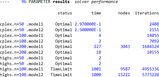
As shown in Figure 1, CPLEX solves the model quickly for each of the parameter lengths. Including the optional constraint (Model 2) is faster than without the optional constraint (Model 1). HiGHS solves for a parameter length 50 items quickly but then struggles to solve the model in a reasonable time for longer parameters (with a time limit of 1,000 seconds). Erwin also tries the Xpress solver, but surprisingly it has numerical issues with the model.

Professor Paul Rubin's results

Paul explores the same situation in the blog post Solver parameters matter.

With default solver options, CPLEX performs much better than Xpress. But after tweaking just one of the several relevant solvers options, Xpress is three or four times faster than CPLEX. The lesson Paul draws is that "...before concluding that one solver is better than another on a problem, or that a problem is too difficult for a particular solver, I need to put a bit of effort into investigating whether any parameter tweaks have substantial impact on performance."

Our approach

We explore another aspect of the same model. Since this is a feasibility problem, we don't need an objective function. But, sometimes, a solver finds an objective function useful anyway. So, we add an arbitrary, though hopefully helpful, objective function to the model to see what difference it makes to the HiGHS solve time performance.

Model formulation

Figure 2 shows the formulation for this model. The formulation is the same as that implemented by Erwin, except we have a choice of objective functions.

Figure 2. Model formulation for sorting a parameter

\begin{alignat*}{1} &\text{Objective}\\ &\quad \text{Minimize} \quad z \quad &= &\quad 0 \quad &&\tag{1a} \\ &\text{Or}\\ &\quad \text{Maximize} \quad z \quad &= &\quad \sum_{i \in I}y_i \times i \quad &&\tag{1b} \\ \\ &\text{Subject to} \\ \\ &\quad \sum_{i \in I}x_{i,j} \quad &= & \quad 1 \quad &\forall j \in I \quad &\tag{2}\\ &\quad \sum_{j \in I}x_{i,j} \quad &= & \quad 1 \quad &\forall i \in I \quad &\tag{3}\\ &\quad y_{i} \quad &= & \quad \sum_{j \in I}x_{i,j} \times \ p_j \quad &&\tag{4}\\ &\quad y_{i} \quad &\geq & \quad y_{i-1} \quad &&\tag{5}\\ &\quad \sum_{i \in I}y_{i} \quad &= & \quad \sum_{i \in I}p_{i} \quad &\text{(Optional)} \quad &&\tag{6}\\ \\ &\text{Variables} \\ &\quad x_{i,j} &= & \quad \text{Permutation matrix, binary} \quad &\forall i,j \in I \quad &\tag{7}\\ &\quad y_{i} &= & \quad \text{Sorted values} \quad &\forall i \in I \quad &\tag{8}\\ \\ &\text{Data} \\ &\quad p_j && \quad \text{Unsorted list of values} \quad &\forall i \in I\quad &\tag{9}\\ \\ &\text{Sets} \\ &\quad I && \quad \text{Position} \quad &i,j = 1..n \quad &\tag{10}\\ \end{alignat*}

The objective function alternatives are:

Equation (1a): A constant of 0. This objective function is minimized, though it can't change so maximization will also work.
Equation (1b): Sum the sorted values variables multiplied by the position of the variables in the list. The idea is that when the list is sorted, this objective function will have its maximum value – since we're sorting in ascending order. Therefore, we maximize this objective function. Minimization will also work – because the optimal solution is unique – though maximization makes more intuitive sense.

We think of Equation (1b) as giving the solver some "traction" in seeking better solutions. That is, having an objective function that improves as the list becomes closer to sorted will – hopefully – help the solver. In this situation, all solutions are infeasible until the unique optimal solution is found, so the solver can use the objective function only as a bound. In other situations, an alternative objective function may lead to faster progress through feasible solutions towards an optimal solution.

Implementation

Parameters to be sorted

We generate a list of uniformly distributed random numbers in the range 0 to 1. To explore how the solve time varies as a function of the number of items in the list, we loop over the model several times. That is, we look at list lengths of 50, 75, 100, 125, 150, 175, and 200 items.

Alternative objective functions

The key part of our model implementation is a choice of objective functions. The Pyomo code for this is shown in Figure 3.

Figure 3. Choice of objective functions

    if OBJ_CHOICE == 1:
        model.obj = pyo.Objective(expr=0, sense=pyo.minimize)
    elif OBJ_CHOICE == 2:
        model.obj = pyo.Objective(expr=sum(model.y[i] * i for i in model.I), sense=pyo.maximize)
    else:
        print('Invalid objective function number')

Model output

Figure 4 shows an example of the model output, when the PRINT_RESULT option is True, given a parameter list of 10 numbers. The original numbers are in random order, while the resulting numbers are sorted in ascending order.

Figure 4. Example model output

Item   Original   Sorted
------------------------
   1     0.6394   0.0250
   2     0.0250   0.0298
   3     0.2750   0.0869
   4     0.2232   0.2232
   5     0.7365   0.2750
   6     0.6767   0.4219
   7     0.8922   0.6394
   8     0.0869   0.6767
   9     0.4219   0.7365
  10     0.0298   0.8922

Comparison of solve times for alternative objective functions

Figure 5 shows the run times (seconds) for our model with the HiGHS solver. We switch off the optional constraint, as HiGHS seems to mostly perform better without it.

For Objective 1a (constant of 0) with a parameter list of 50 items, the model solves in 1.5 seconds. With 75 items, the solve time jumps to over 6 minutes. For the larger lists we allow a solve time of up to 8 hours, but obtain no further solutions (indicated with an "x"). This is consistent with the results reported by Erwin.

For Objective 1b, HiGHS solves all the cases within a few seconds. For the larger list sizes, the alternative objective function takes the model from being intractable to being easily solvable.

Figure 5. Solve times (seconds)

We've previously seen the effect that alternative objective functions can have for performance of feasibility problems. For example, in our article Crossword MILP - Model 2 (section "Alternative objective functions"), we found that using alternative objective functions makes the crossword compilation model up to four times faster to solve.

In the crossword model, the alternative objective functions lead to different solutions, which might matter. But mostly we are looking for any feasible crossword solution, so we don't care about the objective function value or the different solutions. For the sorting model, there is only one solution so the alternative objective functions affect only the solve time performance of the model.

Summary of findings

So, what can we conclude from the models created by Erwin, Paul, and us? The key observations are:

Commercial solvers, like CPLEX, are usually faster than open source solvers like HiGHS. For some models, the performance difference is large.
Solve times may increase exponentially as data size increases. A modest increase in data size can be the difference between a quick solve time and a model that cannot be solved in a reasonable time.
Optional constraints may help. For the parameter list length of 200 items, CPLEX is more than 10 times faster when using the optional constraint. The difference for HiGHS is not so large, and sometimes HiGHS is slower when using the optional constraint. The only way to be sure if an optional constraint will be beneficial is to try it.
Tweaking solver options can have substantial impact on performance, potentially making one solver faster than another.
Even when solving a feasibility problem, sometimes an alternative objective function can help the solver – potentially by a lot.

Conclusion

In this article, we explore the impact of an alternative objective function on solver performance. In this situation, the effect is dramatic, taking the model solve time from being excessive to being solved in seconds.

As Erwin says, "useless models can still be interesting". That's certainly the case here. Although this model isn't likely to be of practical use, we make several observations that may apply more generally, including: optional constraints may help, tweaking solver options can have substantial impact on performance, and sometimes an alternative objective function helps a lot.

If you would like to know more about this model, or you want help with your own models, then please contact us.

Objectives matter: Sorting using a MIP model