Academics, please publish your data and code

2 October 2024

Academic research papers can be a valuable source of material for creating and improving real world optimization models. But, as we have commented previously, we wish that academics would publish working code and data to accompany their papers.

In many papers, the mathematical formulations are poorly defined and hard to understand – often they are just plain wrong. But even when the math is correct, the lack of code and data accompanying most academic papers makes them difficult and time-consuming to replicate, which greatly undermines their value.

Some academic institutions understand the importance and value of publishing data and code, for example:

Reproducible science requires not just sharing the paper and the data, but the methods as well. When those methods are partly or entirely captured by computer code, sharing that code is a powerful step towards making your work fully reproducible. Not only does this allow verification and detailed exploration of your findings, but it also facilitates further research; well-written code can be re-used and even built upon, as a scientific product in and of itself.

Publishing code and software, Utrecht University, The Netherlands

But such a sentiment is an exception rather than the norm.

In this article:

• Firstly, we briefly look at some reasons why academics might be reluctant to publish their data and code.
• Then we replicate, modify, and explore a published model that has been done well, with the data and program code publicly available.

Download the models

The models described in this article are built in Python, using the Pyomo library.

The files are available on GitHub.

Why don't academics share data and code?

A missed opportunity to create value

Operations Research, as a discipline, has existed since just before World War II. In the almost 90 years since then, academic researchers and practitioners have amassed a substantial body of literature covering the theory and practice for formulating and solving a diverse range of problems.

Despite the potentially enormous value contained in the academic literature, much of it is difficult to access. Part of the difficulty is due to the style of academic writing, which typically requires specialized knowledge to even begin to understand what an academic paper says. But even for those with sufficient knowledge, a further difficulty is translating a paper's math into working program code. That's especially true when the math is inadequately, or incorrectly, articulated.

While some academic papers present only theoretical content, many papers describe working models. In the latter case, a common paper structure includes sections that discuss the theoretical background, related research, mathematical formulation of the situation, and results of running the model(s). The part that is often missing is the model implementation used to produce the results – despite the data and code existing.

The omission of data and code makes the models difficult and time-consuming to replicate. In many papers, there is insufficient detail to even attempt a replication. The lack of available data and code greatly undermines the value of many published academic papers. For academic researchers, this is a missed opportunity to have a greater impact.

Barriers, concerns, and disincentives

There are many reasons why academic researchers do not share their data and code. The paper Why don't we share data and code? Perceived barriers and benefits to public archiving practices articulates those reasons very well, so we summarize them below.

The paper's 12 perceived barriers, and the author's proposed solutions, are shown in Figure 1 – followed by a more detailed summary of the reasons.

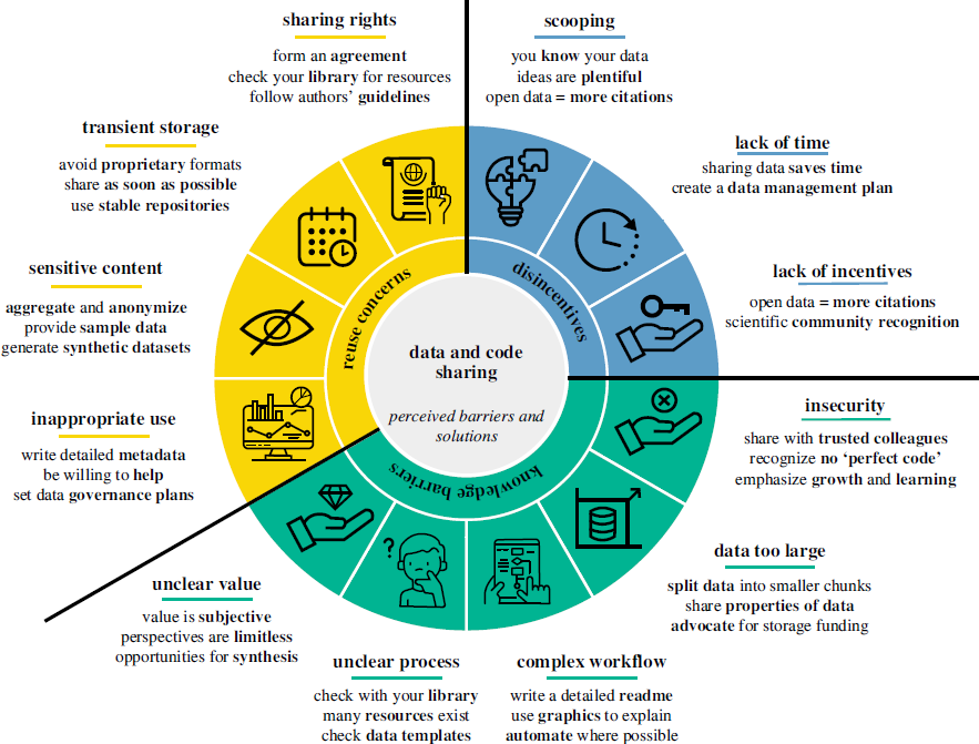
Knowledge barriers:

• Insecurity: Embarrassment, fear, and insecurity can hinder sharing. Seeking feedback from peers, using pre-print servers, and sharing materials during peer review can help. Emphasizing growth and learning over criticism can reduce these insecurities.
• Data too large: Sharing large datasets can be challenging. Cloud storage solutions may offer free storage options. Additionally, data can be divided into subsets for easier management.
• Complex workflow: Workflows may involve manual steps or proprietary software. Automating and documenting these steps can enhance efficiency and reproducibility.
• Unclear process: Researchers may lack knowledge about organizing data and code. Utilizing templates and repositories can be beneficial. Sharing data, even if imperfect, is better than not sharing at all.
• Unclear value: Data and code may be undervalued, especially with small sample sizes or high uncertainty. However, even imperfect data can promote interdisciplinary collaboration and significantly benefit future research.

Reuse concerns:

• Inappropriate use: There may be concerns about data misuse and misinterpretation. Providing contact information, metadata, inviting collaboration, and using permission settings can encourage proper use.
• Sensitive content: Aggregating, anonymizing, or generating synthetic data can mitigate risks associated with sensitive information. Ethical considerations and data sovereignty are crucial.
• Transient storage: Using open repositories can ensure permanence. Avoiding proprietary formats and journal paywalls is recommended.
• Sharing rights: Ownership of data and code can be complicated, involving multiple institutions and funders. Establishing sharing agreements can ensure clarity about sharing rights.

Disincentives:

• Scooping: The fear of being 'scooped' deters researchers from sharing data and code. However, scooping is rare. Pre-print servers can help establish a claim.
• Lack of time: Preparing and supporting data and code can be time-consuming. Good organization from the start can save time in the long run.
• Lack of incentives: Career and reward incentives are often seen as lacking. However, sharing can increase visibility, recognition, and collaboration opportunities, leading to higher citation rates.

Situation

As an example of academic publication done well, we replicate a model described in the paper "Political districting" by Austin Buchanan.

The paper defines political districting as "the task of partitioning a state into geographic-based districts for election purposes". Design of political districts generally requires compliance with multiple criteria, including: equal population (within tolerances), contiguity, communities of interest, etc. Political districting models may be used to reduce the problems associated with partisan gerrymandering.

Models for designing political districts can be applied to a wide range of geographic aggregation situations, like defining franchise territories or facility location problems. Therefore, political districting models can help practitioners solve a variety of business problems. The potential applicability of academic research to a range of practical problems beyond the researcher's original scope is a key reason why the accessibility of data and code from academic papers is so important.

Original implementation

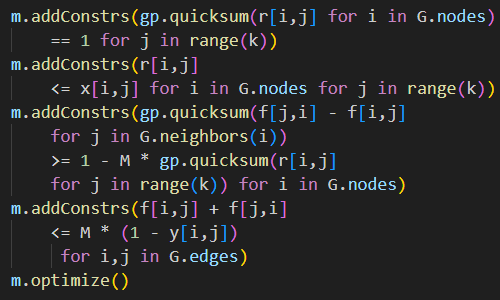
Dr. Buchanan's GitHub repository includes Jupyter Notebooks for several redistricting models and data for the counties of several states. We focus on replicating the "D4-Min-Perimeter-with-Contiguity" model and applying it to the Oklahoma data. Part of that model's code is shown in Figure 2.

# create model 
m = gp.Model()

# create variables
x = m.addVars(G.nodes, k, vtype=GRB.BINARY) # x[i,j] equals one when county i is assigned to district j
y = m.addVars(G.edges, vtype=GRB.BINARY)    # y[u,v] equals one when edge {u,v} is cut

# objective is to minimize weighted cut edges (district perimeter lengths)
m.setObjective( gp.quicksum( G.edges[u,v]['shared_perim'] * y[u,v] for u,v in G.edges ), GRB.MINIMIZE )

# add constraints saying that each county i is assigned to one district
m.addConstrs( gp.quicksum( x[i,j] for j in range(k)) == 1 for i in G.nodes )

# add constraints saying that each district has population at least L and at most U
m.addConstrs( gp.quicksum( G.nodes[i]['TOTPOP'] * x[i,j] for i in G.nodes) >= L for j in range(k) )
m.addConstrs( gp.quicksum( G.nodes[i]['TOTPOP'] * x[i,j] for i in G.nodes) <= U for j in range(k) )

# add constraints saying that edge {u,v} is cut if u is assigned to district j but v is not.
m.addConstrs( x[u,j] - x[v,j] <= y[u,v] for u,v in G.edges for j in range(k) )

m.update()

# Now, let's add contiguity constraints and re-solve the model.
# We will use the contiguity constraints of Hojny et al. (MPC, 2021)
#   https://link.springer.com/article/10.1007/s12532-020-00186-3

# Add root variables: r[i,j] equals 1 if node i is the "root" of district j
r = m.addVars( G.nodes, k, vtype=GRB.BINARY)

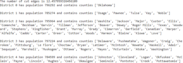
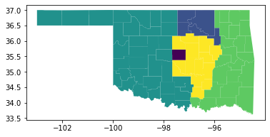
The original model's printed output, as shown in Figure 3, lists the counties that have been aggregated into districts and shows that the districts have approximately equal populations. A map of the model's solution, as shown in Figure 4, shows how the counties of Oklahoma are aggregated into five contiguous electoral districts.

Replication and modification of the model

Implementing the model would be challenging without the code and data

The various papers describing the political districting models provide good descriptions of the formulations. Therefore, it would be reasonably straightforward, though time-consuming, to express the model in Pyomo given just the papers.

A greater challenge would be creating the required data, which is quite extensive. The map data is especially complex. In addition, writing the code to do the mapping would not be straightforward if the modeller is unfamiliar with the mapping library.

Having working code and an example data set greatly simplifies the process of replicating the original model.

Translate from gurobipy to Pyomo

As is often the way with academic optimization models, Dr. Buchanan uses the commercial Gurobi solver – presumedly because academics can get free licences. The code is written using Gurobi's proprietary library gurobipy, which is designed specifically for the Gurobi solver.

With a Gurobi solver license, we could run the original model code as is. However, Gurobi licenses are quite expensive, and many practitioners do not have access to a Gurobi license. In addition, the gurobipy code is specific is the Gurobi solver, while we prefer the more general Pyomo library – partly because it allows us to use different solvers (including Gurobi).

So, we want to translate the original code to use the Pyomo library and the HiGHS solver. Fortunately, Large Language Model Artificial Intelligence (LLM AI) tools are quite good at performing this type of translation. Therefore, we ask the Windows 11 Copilot AI to translate the gurobipy code to use Pyomo. It does so with only a couple of minor issues, which are easily fixed. Within a few minutes we have a working version of the model using Pyomo and the HiGHS solver.

Part of our model code is shown in Figure 5. The main differences from the original code relate to translating gurobipy syntax to Pyomo syntax.

model = pyo.ConcreteModel()
model.nodes = pyo.Set(initialize=list(graph.nodes()))
model.edges = pyo.Set(initialize=list(graph.edges()))
model.districts = pyo.RangeSet(0, NUM_DISTRICTS-1)
model.assign = pyo.Var(model.nodes, model.districts, within=pyo.Binary)   # Equals one when county i is assigned to district j (originally x)
model.cut = pyo.Var(model.edges, within=pyo.Binary)   # Equals one when edge {u,v} is cut (originally y)
model.root = pyo.Var(model.nodes, model.districts, within=pyo.Binary)   # Equals 1 if node i is the "root" of district j (originally r)
DG = nx.DiGraph(graph)
model.directed_edges = pyo.Set(initialize=list(DG.edges()))
model.flow = pyo.Var(model.directed_edges)
model.objective = pyo.Objective(rule=lambda model: sum(graph.edges[u, v]['shared_perim'] * model.cut[u, v] for u, v in model.edges), sense=pyo.minimize)
model.one_district = pyo.Constraint(model.nodes, rule=lambda model, i: sum(model.assign[i, j] for j in model.districts) == 1)
model.population_lower = pyo.Constraint(model.districts, rule=lambda model, j: sum(graph.nodes[i]['TOTPOP'] * model.assign[i, j] for i in model.nodes) >= pop_lb)
model.population_upper = pyo.Constraint(model.districts, rule=lambda model, j: sum(graph.nodes[i]['TOTPOP'] * model.assign[i, j] for i in model.nodes) <= pop_ub)
model.cut_edge = pyo.Constraint(model.edges, model.districts, rule=lambda model, u, v, j: model.assign[u, j] - model.assign[v, j] <= model.cut[u, v])
model.one_root = pyo.Constraint(model.districts, rule=lambda model, j: sum(model.root[i, j] for i in model.nodes) == 1)
model.root_assignment = pyo.Constraint(model.nodes, model.districts, rule=lambda model, i, j: model.root[i, j] <= model.assign[i, j])
M = graph.number_of_nodes() - NUM_DISTRICTS + 1
model.flow_conservation = pyo.Constraint(model.nodes, rule=lambda model, i: (sum(model.flow[j, i] for j in graph.neighbors(i)) \
   - sum(model.flow[i, j] for j in graph.neighbors(i))) >= 1 - M * sum(model.root[i, j] for j in model.districts))
model.no_flow_cut_edge = pyo.Constraint(model.edges, rule=lambda model, i, j: model.flow[i, j] + model.flow[j, i] <= M * (1 - model.cut[i, j]))
return model

Modify the model to suit our purpose

Having a working model enables us to explore the model's behaviour with a variety of settings, data sets, and solvers. This helps us enhance our understanding of the model to a much greater extent than we could by just reading the published papers.

We can also modify the model to suit our purpose. That might be applying the model to a different jurisdiction's political districting situation, or it might be using the model as a basis for a different situation such as defining franchise territories for a business.

In this case, we modify the translated model as follows:

• Modularize the code by using functions, to make the code easier to understand and maintain.
• Expand the printed results to show additional detail and use a nicer format.
• Enhance the result map by adding markers that indicate the location of optionally specified "root counties" (the counties that the districts may be built around).
• Add a map showing the population of each county, to help us understand the solution.
• Rename some objects to use more meaningful names. For example, change one-letter names like G and k to graph and NUM_DISTRICTS respectively.

Translating the model and making these changes takes less than an hour. If we had access to only the published papers, then writing code and creating data would have taken many times longer.

Results from the modified model

When seeking to create five districts in Oklahoma, our modified model finds the same solution as that described in the papers. The printed output from our modified model is shown in Figure 6. In addition to reformatting the output, we've added the deviation for each district – reflecting the constraint that each district's population must be within ±1% of the total state's population divided by the number of districts.

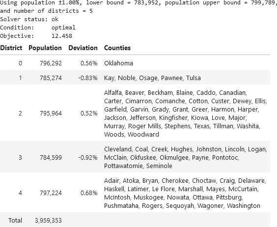
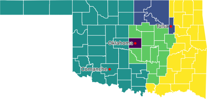
Figure 7 shows a map of Oklahoma, as produced by our modified model, indicating the aggregation of the counties into five voting districts. We specified three root counties, as marked on the map. This allocation of counties to districts is the same as that produced by the original model.

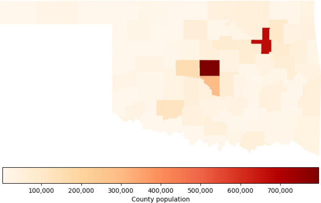
Since political districting is a geographic problem, maps are especially important. Having the original model's data and code for creating the allocation map greatly simplifies the process of adding a map of county population, as shown in Figure 8. This map makes it clear that a substantial portion of Oklahoma's population resides in Oklahoma County and Tulsa County, with most of the state being relatively sparsely populated rural counties.

Finding an optimal solution is slower when using the HiGHS solver compared with the Gurobi solver. That is expected, as the commercial Gurobi solver is usually faster than the free, open-source HiGHS solver. Nonetheless, the HiGHS solver is good enough to solve the model in a reasonable time – between a few seconds and a few minutes, depending on the parameters.

Exploring use of the model

Let's make three districts

With a working model and data, we can explore how the model behaves with different inputs. For example, suppose we want to divide Oklahoma into three districts instead of five districts? We simply change the NUM_DISTRICTS parameter to equal 3 and re-run the model. The result is shown in Figure 9.

This solution is surprising. The districts are not all contiguous, even though we have constraints to create contiguous districts. It seems that we have an error in our model.

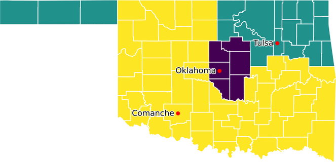
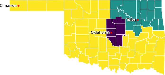
To create three contiguous districts, we change one of the root counties from Comanche to Cimarron. The result is shown in Figure 10. To comply with the population bounds, the model has swapped Cimarron and adjacent counties for one of the counties that was part of the Tulsa district. The result is three contiguous districts, as required.

Correcting our model

Although we have a contiguous solution for three districts, we haven't addressed the issue that our model is wrong.

Recall that the original model was translated by Copilot, so perhaps it made an error – as it occasionally does. To be fair, manually translating the model would also be potentially error-prone, so we can't blame Copilot if it did make an error.

Despite gurobipy and Pyomo having different syntax, there is a roughly one-to-one relationship between the two libraries. This makes the translation process easier. Careful manual comparison of the original gurobipy implementation with our Pyomo implementation confirms that the translation is accurate. So there must be some other issue.

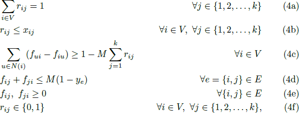
We have a look at the published papers that describe the districting models, including Imposing contiguity constraints in political districting models and IEM 4013: Two MIPs for redistricting. The latter paper describes the formulation for ensuring contiguous districts as implemented in the model we're replicating. That formulation is shown in Figure 11.

Both the gurobipy and Pyomo models accurately reflect this formulation – except for one detail: Constraint (4e) requires the flow variables to be non-negative. Neither model explicitly enforces this requirement.

To see what's happening, we re-run our Pyomo model and print the values of the flow variables using model.flow.pprint(). This shows that some of the flow variables are negative, which is not supposed to happen.

The issue is that gurobipy assumes variables are non-negative unless specified otherwise, while Pyomo does not make that assumption. Copilot correctly translated the original model as stated, but it didn't add the unstated non-negativity requirement – a subtle, though understandable, error. It is probably asking too much from Copilot to expect that it would add something that isn't in the source material.

To fix the error in our model, we change the definition of the flow variables to specify that they are non-negative. That is, model.flow = pyo.Var(model.directed_edges, within=pyo.NonNegativeReals). It is good practice to always specify the domain of variables, so that's an oversight we should have corrected when checking Copilot's translation.

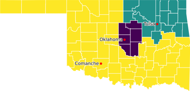
Re-running the model, after reverting to having Comanche as a root county, produces the result shown in Figure 12. We now have three contiguous districts, as expected. Therefore, we're happy that we've fixed that error in our Pyomo model.

This error was easy to identify and fix. But if we had to write the code and create the data, using only the published papers, then it is almost certain that there would be more errors. Those errors would likely be time-consuming and frustrating to find and fix. Starting with working code and data helps enormously.

Conclusion

In this article, we implore academics to publish data and code to accompany their papers. Having the data and code makes replication and extension so much easier. Conversely, failing to publish data and code greatly undermines the value of academic papers.

To illustrate the point, we replicate a political redistricting model where the data and code are published. Given the complexity of the formulation and especially the data, replicating this model solely from the published papers would have been difficult and time consuming.

But given all the published information, we're able to quickly translate the original model code to use our preferred tools. We then replicate the original results using the available data. With a working model, we make some modifications to suit our purpose. Then we explore alternative solutions – discovering an error in our model, which we're able to correct by referring to the formulation in one of the published papers.

Academic papers are a tremendously valuable resource, for both learning and solving real problems. But much of that value can only be realized if practitioners, like us, can use the knowledge in those papers. So, academics, please publish your data and code.

If you would like to know more about this model, or you want help with your own models, then please contact us.

References

Buchanan, A. (2022). IEM 4013: Two MIPs for redistricting, GitHub repository https://github.com/AustinLBuchanan/Districting-Examples-2020

Buchanan, A. (2023). Political districting, in Pardalos, P.M., Prokopyev, O.A. (eds) Encyclopedia of Optimization. Springer, Cham. Page 1-9.

Gomes, D. G. E., et al. (2022). Why don't we share data and code? Perceived barriers and benefits to public archiving practices, Proceedings of the Royal Society B: Biological Sciences, 289.

Validi, H., Buchanan, A., and Lykhovyd, E. (2022). Imposing contiguity constraints in political districting models, Operations Research, 70(2), 867-892.