13 August 2024

We continue our exploration of methods to solve our device rack positioning problem. The methods are:
- Model 1. Enumerate all possible position orders.
- Model 2. Search randomly for a specified time.
- Model 3. Local search around random starting positions.
- Model 4. Constraint programming using OR-Tools.
- Model 5. Mixed integer linear programming using Pyomo.
The previous article describes Model 2, which uses a parallel random search method to find good solutions. Model 2 works surprisingly well, even for the larger data sets, finding solutions that are up to 50% better than those we found by partial enumeration in Model 1.
In this article, we develop Model 3, which implements a variation of the random search method. We start with a solution (initially random), then swap the positions of a pair of devices. If that solution is better, then it becomes the incumbent solution and we repeat the process, otherwise we keep swapping positions in the initial solution. In effect, this process is a simple heuristic for searching the solution space around a solution. This method, known as a "local search", has the potential to improve the initial solutions. Will local search perform better than a pure random search in this situation?
Download the models
The models described in this series of articles are built in Python.
The files are available on GitHub.
Situation
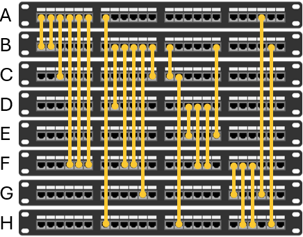
The situation is described fully in the first article of this series. Briefly, we have network devices in a rack. We need to use cables to connect each device to one or more other devices in the rack, arranged like in Figure 1. The question is, in what order should we position the devices to minimize the total cable length?
Model 3 design
We start with Model 2 and make some fairly minor changes. Specifically, after generating a random solution, we swap the positions of two randomly chosen devices to see if that produces a better solution. If it does, then we use that solution as the basis for making more swaps. Otherwise, we make more swaps in the initial solution.
Like Model 2, Model 3 runs the search process in parallel, using all the CPU's available cores/threads. At a specified interval, we share the best solution found so far across all the cores/threads. By itself, this standardization of solutions might lead to stagnation as all cores/threads work on very similar parts of the solution space. To prevent that and mitigate the possibility that the initial solutions are not good, we also occasionally refresh a proportion of the cores/threads with new random solutions.
The model loops for a specified time, doing a local search around existing solutions and generating new random solutions. At the end of the time limit, the model reports the best solution found. The reported %done represents the elapsed percentage of the time limit.
This local search method is very simple. There are certainly many ways in which it could be improved. Our goal is to illustrate a program structure, including parallel processing with communication between processes, that could be used as the basis for more sophisticated local search models. For example, OR-Tools (which we'll use in the next article) uses more sophisticated local search heuristics in its toolkit of methods.
Model 3 implementation
Data structure
Model 3 uses the same input data structure used by Models 1 and 2.
Differences from Model 2
We start with the code for Model 2 and make two key changes to produce Model 3.
First, we copy the current incumbent best order and swap the positions of two devices. After doing the swap, we identify whether the swap produces a better solution (shorter total length of cable). If it does, then the new solution becomes the incumbent on which we perform more position swaps. The code for doing this is shown in Figure 2. This code is run in parallel by each core/thread.
new_order = copy.deepcopy(order[:])
i, j = random.sample(range(num_devices), 2)
new_order[i], new_order[j] = new_order[j], new_order[i]
new_length = calculate_total_length(new_order, cable_struct)
if new_length < min_length:
    order = copy.deepcopy(new_order)
    local_best_case = copy.deepcopy(new_order)
    min_length = new_length
Second, every RESTART_INTERVAL seconds, we either share the best solution from all threads with the current thread, or we generate a new random solution. The choice of which step to take is random, given a fixed probability. This process is run by each parallel thread. The code for doing this step is shown in Figure 3.
if current_time - last_restart >= RESTART_INTERVAL:   # Potentially restart with a new random order every RESTART_INTERVAL seconds
    if random.random() <= RESTART_PROBABILITY:
        random.shuffle(order)
    else:
        order = copy.deepcopy(shared_dict['best_case'])
    last_restart = current_time
Performance of Model 3
Model 3 is more complex than Model 2, so it runs at about half the rate of Model 2. Even so, for the smaller data sets it does about 3 million iterations per second on a 28 core/thread PC, so we're able to assess a good number of device combinations in the time limit of 1 hour.
Example of local search
Figure 4 shows an example of how the local search heuristic improves the solution. We start with a random order for eight devices. This initial solution has a length of 65, which is close to the average of 69 for the distribution of all solutions for eight devices shown in the previous article.
The model then randomly swaps the positions of two devices, until it finds a solution that has a shorter length. In this example, it takes only two iterations to improve the initial random order, swapping devices A and B to find a solution with length 63. We then repeat the process, starting with the most recently found best solution. After five more swaps the length has been reduced to 46 – which we know is optimal for this eight device data.
Iteration   Length   Device order      Description
------------------------------------------------------------
     0        65     E A C H F B G D   Initial random order
     2        63     E B C H F A G D   Swap A and B
     9        59     E C B H F A G D   Swap B and C
    13        57     E C F H B A G D   Swap B and F
    14        53     E D F H B A G C   Swap C and D
    23        47     E D G H B A F C   Swap F and G
    71        46     E D G F B A H C   Swap F and H, optimal
In this example, it took 71 iterations to get from a near-average solution to an optimal solution – though only six of the 71 iterations produced an improved solution. Considering that the model does millions of swaps per second, this is remarkably good. In general, as the model approaches an optimal solution, fewer and fewer of the swaps produce an improvement because better solutions become increasingly rare.
Note that the optimal solution has only one device (E) in its initial position. All the other devices have been swapped at least once, with B and F each being swapped three times. Although our local search heuristic is simple, it is effective in this situation.
Model 3 results
Model output
Figure 5 shows an example of the model output when running the data for 12 devices with a time limit of 30 seconds.
Model 3 finds the optimal solution of length 60 decimetres within 5 seconds. Since the local search has a random element, there's no guarantee of finding a good solution within a reasonable time. But, in practice, Model 3 usually performs much better than Model 2.
Model 3: Cable length management, local search in parallel

     Time    %done     Best
---------------------------
        5   17.25%     75 *
        5   17.27%     62 *
        5   17.32%     61 *
        5   17.32%     61
        5   17.38%     61
        5   17.38%     60 *
        5   17.40%     60
        5   17.68%     60
       10   34.05%     60
       10   34.07%     60
       10   34.35%     60
[...]
       25   84.33%     60
       25   84.35%     60

Devices: 12
Minimum length: 60
Best case: ['L', 'C', 'K', 'H', 'B', 'A', 'F', 'D', 'G', 'I', 'E', 'J']
Rate: 2,374,959 orders per second
Time: 30.04 seconds
Comparison between methods
In Figure 6 we compare the best solutions found by Model 3 with the best solutions found by Models 1 and 2. All models were able to run for up to 1 hour for each data set (number of devices).
Within a few seconds of run time, Model 3 replicates the optimal solutions for 8 to 12 devices, as found by Models 1 and 2. For 13 to 15 devices, Model 3 finds the same objective function values found by Model 2 (though not necessarily the same solutions, as there are alternative optima in each case).
Importantly, the local search method of Model 3 finds better solutions for 16 to 24 devices – by 27% for the 24 device case. In most model runs these solutions are found in a few seconds, though the larger cases sometimes take up to a few minutes.
Allowing the local search to continue for up to 1 hour provides no further improvement in any of the solutions. This doesn't necessarily mean that we've found optimal solutions – that might be true, or perhaps optimal solutions are exceedingly rare and difficult to find for the larger cases.
Model 3's local search heuristic performs materially better than Model 2's pure random search. This isn't surprising. In Model 2, when we randomly generate a good solution, we simply note it and move on to generate a new random solution. That is, having found a good solution, Model 2 doesn't make use of that information.
Conversely, Model 3 assumes that small changes to a good solution might lead to an even better solution. So, we use the information we have, albeit in a very simple manner of randomly swapping two devices. We also share the best solutions across the cores/threads, giving the model a greater chance of finding better solutions. To ensure that we don't get stuck at a local optima, we occasionally mix up the pool of solutions with new random orders. The overall effect is that Model 3's local search method finds much better solutions than Model 2 finds with just random search.
Next steps
By using a local search method, we've been able to significantly improve the solutions for the larger data sets. But, because the solutions are not proven optimal, perhaps we can improve the solutions further?
So, in the next article, we try to find improved solutions by applying Constraint Programming to this problem. The source for this problem used the CPMpy Constraint Programming library. We'll adopt a similar approach, translated to use the OR-Tools library.
Conclusion
In this article, we use a local search method to find improved solutions to our problem of positioning devices in a rack. Model 3's parallel local search heuristic works very well. It is much better than Model 2's pure random search method.
Even though we have better solutions for the larger device cases, none of those solutions have been proven optimal. It might be possible to do even better by using a more sophisticated method. Therefore, in the next article, we formulate the situation as a Constraint Programming problem and solve it using the CP-SAT solver in OR-Tools.
If you would like to know more about this model, or you want help with your own models, then please contact us.


