12 September 2024

We complete an exploration of methods to solve our device rack positioning problem. The methods are:
- Model 1. Enumerate all possible position orders.
- Model 2. Search randomly for a specified time.
- Model 3. Local search around random starting positions.
- Model 4. Constraint programming using OR-Tools.
- Model 5. Mixed integer linear programming using Pyomo.
Of the models we've looked at so far, the constraint programming method works best. Model 4 quickly finds optimal solutions for all cases except the largest (24 device) case. Even then, its solution for the 24 device case is probably optimal.
In this article, we develop Model 5, which formulates the situation as a Mixed Integer Linear Program (MILP) in Pyomo. Will this method work as well as constraint programming, or perhaps even better?
Download the models
The models described in this series of articles are built in Python.
The files are available on GitHub.
Situation
The situation is described fully in the article for Model 1. Briefly, we have network devices in a rack. We need to use cables to connect each device to one or more other devices in the rack, arranged vertically. The question is, in what order should we position the devices to minimize the total cable length?
Model 5 design
The previous article solved this situation using constraint programming in OR-Tools. That model uses two features that are easy to implement in constraint programming:
- All Different. Each of the devices is required to occuply a different position in the rack.
- Absolute Value. The length of cable is positive irrespective of the order of the devices.
We're using the HiGHS solver, so our model need to be linear. But Pyomo does not have native All Different and Absolute Value features, at least in a linear formulation. Therefore, we need to create linear constraints that produce equivalent behaviours in our model.

All Different
There are several methods for making variables all have different values from a discrete set – such as the position of devices in a rack.
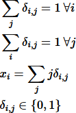
In this case, our situation matches Approach 2 described at All-different and mixed integer programming. That is, the devices can be in position 1 to n, with each device in a different position. The math for this approach is shown in Figure 1, which uses an n by n matrix of binary variables to represent each combination of positions.
Note that it is possible to drop one of the first two constraints. It doesn't seem to make a material difference in this model so, for completeness, we leave the constraints as is.

Absolute Value
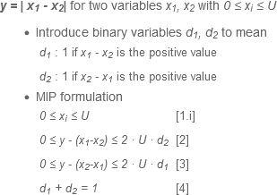
Representing an absolute value linearly is a bit more complex. We use the method described at Absolute Values.
That is, we define binary variables to represent the positive and negative values, then constrain them represent the absolute values and ensure that only one outcome is binding at a time. The math for this approach is shown in Figure 2.
Formulation for Model 5
We convert the formulation for the previous constraint programming model to be a Mixed Integer Linear Program (MILP). The key differences relate to representing the All Different and Absolute Value constraints as described above. The resulting MILP formulation is shown in Figure 3.
Model 5 implementation
Data structure
Model 5 uses the same input data structure used by the previous models.
Formulation code
The code for implementing this formulation, part of which is shown in Figure 4, is much longer than the constraint programming version. That's because we need to use multiple constraints and additional variables to represent the All Different and Absolute Value aspects, rather than using built-in features like we can with OR-Tools..
    def rule_position_allocation(model, p):   # Allocate each device to a unique position in the rack
        return model.Allocation[p] == sum(q * model.AllDiff[p, q] for q in model.Position)
    model.PositionAllocation = pyo.Constraint(model.Position, rule=rule_position_allocation)

    def rule_diff1(model, p):   # All Different constraint, part 1
        return sum(model.AllDiff[p, q] for q in model.Position) == 1
    model.Diff1 = pyo.Constraint(model.Position, rule=rule_diff1)

    def rule_diff2(model, q):   # All Different constraint, part 2
        return sum(model.AllDiff[p, q] for p in model.Position) == 1
    model.Diff2 = pyo.Constraint(model.Position, rule=rule_diff2)
Two versions of Model 5
Just for fun, we implement two versions of Model 5:
- Model 5a. A standard implementation except that we create a model file locally and then run it using the Gurobi solver on NEOS Server.
- Model 5b. Uses the multiprocessing library to call multiple instances of the local HiGHS solver in parallel.
Model 5a: Gurobi
HiGHS struggles to consistently produce good results with this model, so our Pyomo code writes the model to a file (in GAMS format) and we run it manually on NEOS Server using the Gurobi solver. We need to run the model manually because, unlike many other solvers, Gurobi is not accessible remotely.
For Model 5a, we haven't found a way to make Pyomo include the time limit in the output GAMS model file. Therefore, we manually edit the GAMS file to include the reslim option with a value of 3600 seconds, as shown in Figure 5. This limits the Gurobi solve time to 1 hour.
MODEL GAMS_MODEL /all/ ;
option solprint=off;
option limrow=0;
option limcol=0;
option solvelink=5;
option reslim=3600;
SOLVE GAMS_MODEL USING mip minimizing GAMS_OBJECTIVE;
Model 5b: Parallel instances of HiGHS
For Model 5b, the code for running parallel instances is largely the same as for Model 5a. The key difference is that we create a pool of processes, each of which independently runs the model with the HiGHS solver.
Each instance has a different random seed value, defined using the solver options:
solver.options['random_seed'] = rd.randrange(2**31) - 1
The random seed changes some choices that the solver makes, leading to different solutions. HiGHS is mostly single-threaded, so on our 28 thread/core CPU, running 16 instances of the model keeps the CPU close to 100% utilization. Each model instance is fairly small, so RAM usage is not a concern.
We collate the results from each instance and print the best solution found. The model formulation is identical in both versions of the model. Most of the code for creating the threads and running of them is shown in Figure 6. There are a few other minor, but important, differences in other parts of the code.
def run_model_thread(lock, thread_id):   # Create and run a single thread
    start_time = tm.time()
    model = pyo.ConcreteModel(name=f"{MODEL_NAME} - Thread {thread_id}")
    num_connections, num_devices, max_diff, length_lb = get_data()
    model.Engine = SOLVER_NAME
    model.TimeLimit = TIME_LIMIT
    solver, model = set_up_solver(model, thread_id)
    model = define_model_data(model, num_connections, num_devices, max_diff, length_lb)
    model = define_model(model)
    if WRITE_MODEL_FILE:
        model.write(f'Model_thread_{thread_id}.gams', io_options={'symbolic_solver_labels': False})
    results = call_solver(solver, model)
    write_solution, condition = check_solution(model, results)
    end_time = tm.time()
    elapsed_time = end_time - start_time
    with lock:   # Acquire thread lock so that different threads don't print simultaneously
        objective_value, best_case = write_thread_solution(model, write_solution, thread_id, condition, elapsed_time)
    return thread_id, condition, objective_value, best_case, elapsed_time

  def main(threads):   # Run the model
    print(MODEL_NAME, '\n')
    with mp.Manager() as manager:   # Create manager to pass lock to threads; necessary on Windows
        lock = manager.Lock()
        with mp.Pool(processes=mp.cpu_count()) as pool:
            results = [pool.apply_async(run_model_thread, (lock, i,)) for i in range(threads)]
            all_results = [result.get() for result in results]
        all_results.sort(key=lambda x: x[0])  # Sort results by thread_id
        write_summary(all_results)
Model 5 results
Model 5a, Gurobi
Using the Gurobi solver on NEOS Server, running with a 1 hour time limit, we find proven optimal solutions for the smaller cases and good solutions for the larger cases. The objective function values are the same as we found with the Constraint Programming model, except for the case with 18 devices which is 1 decimetre longer. Therefore, apart from 18 devices, the solutions are optimal – though none of the cases for 18 or more devices is proven optimal by Gurobi.
In terms of performance, Gurobi's convergence towards optimality is much slower than the OR-Tools Constraint Programming Model 4. It isn't surprising that the Constraint Programming model performs better than the MILP model in this situation. Constraint Programming is better suited to finding good/optimal solutions for this model, given that it can natively handle our All Different and Absolute Value requirements. Conversely, we need to jump through some hoops to create an equivalent formulation in our MILP model.
Model 5b, HiGHS in parallel
Running 16 instances of the HiGHS solver in parallel achieves about the same performance as using Gurobi with Model 5a (though Gurobi is limited to 4 threads when running on NEOS Server). That is, the best solutions found have the same objective function values as we previously found with the Constraint Programming model, except for a couple of cases that are 1 decimetre longer (specifically, 20 and 22 devices). Again, the smaller cases are proven optimal, while the larger cases find optimal solutions but none are proven optimal within the 1 hour time limit.
Figure 7 shows a summary of the results from running the 24 device data with Model 5b using 16 instances of HiGHS and a time limit of 3600 seconds. The threads produce a variety of objective function values. Two threads find an objective function value of 130, which is the optimum though the solver did not prove that in these threads. The worst thread result has an objective function value of 153, which is 18% higher than the optimal result.
Thread     Status          Seconds    Objective
-----------------------------------------------
   0       maxTimeLimit    3600.6           134
   1       maxTimeLimit    3600.5           131
   2       maxTimeLimit    3600.6           150
   3       maxTimeLimit    3600.6           130
   4       maxTimeLimit    3600.7           135
   5       maxTimeLimit    3600.6           130
   6       maxTimeLimit    3600.5           153
   7       maxTimeLimit    3600.7           148
   8       maxTimeLimit    3600.7           149
   9       maxTimeLimit    3600.7           147
  10       maxTimeLimit    3600.5           142
  11       maxTimeLimit    3600.5           145
  12       maxTimeLimit    3600.6           151
  13       maxTimeLimit    3600.7           143
  14       maxTimeLimit    3600.6           140
  15       maxTimeLimit    3600.5           149
-----------------------------------------------
The point of running multiple instances of the solver in parallel is that we're more likely to get a good solution. That is, when running one thread, we might be lucky and get a good solution. With multiple threads we increase the odds of getting a good, perhaps optimal, solution.
Conclusion
In this article, we solve our cabling problem using a Mixed Integer Linear Programming (MILP) model in Pyomo.
This model finds good solutions – either the same, or within 1 decimetre, as those we found using a Constraint Programming (CP) model. But our MILP model is much slower than our CP model. The CP model finds optimal or probably optimal solutions in less than 1 second for all of our cases. The MILP model takes minutes or tens of minutes to find similar solutions. The difference in performance isn't surprising, as CP is especially well suited for this situation.
In other situations, a MILP model may be better than a CP model. Often, the only way to be sure which method will work better is to build the models and see what happens.
Model 5b is especially interesting, as running multiple instances of the HiGHS solver in parallel achieves about the same performance as using the Gurobi solver. Gurobi, which is natively multi-threaded, is usually faster than the mostly single-threaded HiGHS solver. Our method closes some of that performance gap. There are plans to implement a parallel version of the HiGHS solver. But, in the meantime, running multiple instances of HiGHS in parallel with different random number seeds is a useful technique.
If you would like to know more about this model, or you want help with your own models, then please contact us.


