Well, that escalated quickly: OR-Tools

26 August 2024

We continue our exploration of methods to solve our device rack positioning problem. The methods are:

• Model 1. Enumerate all possible position orders.
• Model 2. Search randomly for a specified time.
• Model 3. Local search around random starting positions.
• Model 4. Constraint programming using OR-Tools.
• Model 5. Mixed integer linear programming using Pyomo.

The previous articles describe the enumeration and parallel random search methods. Enumeration finds optimal solutions for the small data sets, but performs poorly for larger data sets. The random search method finds good solutions for the larger data sets, but those solutions are unlikely to be optimal. Using a more focussed local search method, we improved the solutions even further.

In this article, we develop Model 4 which formulates the situation as a Constraint Programming problem and solves it using the CP-SAT solver in OR-Tools. Perhaps this more sophisticated method will enable us to find optimal solutions for all of our data sets?

Download the models

The models described in this series of articles are built in Python.

The files are available on GitHub.

Situation

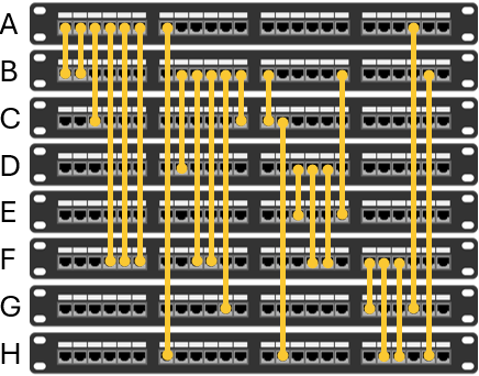
The situation is described fully in the article for Model 1. Briefly, we have network devices in a rack. We need to use cables to connect each device to one or more other devices in the rack, arranged like in Figure 1. The question is, in what order should we position the devices to minimize the total cable length?

Model 4 design

The source for this problem used the CPMpy Constraint Programming library. We adopt a similar approach, translating that model to use the CP-SAT solver in OR-Tools.

Formulation for Model 4

Our problem situation is quite simple. We require each device to occupy a unique position in the rack. Given the positions, we calculate the length of cable needed to make the required connections between devices. Our objective is to minimize the total cable length.

Compared with linear programming solvers, constraint programming solvers generally include a wider range of formulation mechanisms. In this situation, we can take advantage of two mechanisms that are often especially useful:

• All different constraint. We specify the device positions using the AddAllDifferent() function. This requires each of the device positions to be a different integer from 0 to n.
• Absolute value function. The objective function is the total length of cable between devices. We use the absolute value function, AddAbsEquality(), to ensure the cable length is positive irrespective of the device positions.

Model 4 implementation

Data structure

Model 4 uses the same input data structure used by the previous models in this series.

Formulation code

The code for implementing this formulation is straightforward, as shown in Figure 2. The code includes an option for returning either the best solution found (designated as Phase 1) or all optimal solutions.

def Formulation(cable_struct, num_connections, num_devices, max_diff, phase_1, best, length_lb):
    model = cp_model.CpModel()

    connection_list = pd.RangeIndex(num_connections)
    device_list = pd.RangeIndex(num_devices)
    position = model.NewIntVarSeries(index = device_list, lower_bounds = 0, upper_bounds = num_devices - 1, name = "Position")
    length = model.NewIntVarSeries(index = connection_list, lower_bounds = 0, upper_bounds = max_diff, name = "Length")
    
    model.AddAllDifferent(position)   # The devices must occupy different positions in the rack

    for i, (device_from, device_to, cables) in enumerate(cable_struct):    # Cable length between devices
        model.AddAbsEquality(length[i], (position[device_from] - position[device_to]) * cables)   # Note the absolute value used for calculating length

    model.Add(sum(length) >= length_lb)   # Additional constraint, lower bound if all lengths are 1
    
    if phase_1:
        model.Minimize(sum(length))   # In Phase 1, minimize the total cable length
    else:
        model.Add(sum(length) == best)   # For subsequent runs, find solutions with cable length found in Phase 1

    return model, position, length, connection_list, device_list

We also include an additional constraint: a lower bound on the objective function, assuming all cable lengths are 1 (which they must be, at least). It is not clear if this constraint helps the solver, though it doesn't seem to do any harm.

Model 4 results

Comparison between methods

In Figure 3 we compare the best solutions found by the model so far. All models ran for up to 1 hour for each data set (number of devices).

Model 1 already found optimal solutions for 8 to 12 devices by enumerating all possible device orders. Model 4 confirms that the solutions found by Model 2's random search are optimal for 13 to 15 devices. Model 4's run time to find those solutions is less than 1 second, though proving optimality takes between 8 and 30 seconds.

For 16 to 22 devices, Model 4 finds solutions that are proven to be optimal, confirming that Model 3 found optimal solutions for those cases. All solutions are found within 1 second, though it takes progressively longer to confirm optimality (up to 37 minutes for 22 devices).

Model 4's solutions for 23 and 24 devices are also found within 1 second, but optimality is not proven within the 1 hour time limit. The solutions are the same as those solution found by Model 3. Running Model 4 with a longer time limit proved optimality for the 23 device data in 2.8 hours, but optimality was not proven for the 24 device data in 15 hours. Even so, the solution for 24 devices is probably optimal.

Performance of the constraint programming solver

The performance of the OR-Tools CP-SAT solver is remarkable. Each of the solutions is found within 1 second, though it takes longer to prove optimality. In most practical situations, finding a good solution is much more important than proving optimality. Therefore, solving all of the data sets within 1 second is an excellent performance.

Given the enormous size of the solution space for the larger data sets, Model 4 demonstrates how powerful the constraint programming method can be. Recall from the first article that enumerating all cases for the 24 device data set would take more than six times the current age of the universe. Yet the constraint programming solver found an excellent (probably optimal) solution in less than 1 second. With the right tool, and contrary to popular belief, a combinatorial explosion may not be much of a barrier after all.

Finding alternative optima

The OR-Tools CP-SAT solver has a useful feature that enables it to find alternative optima. In Model 4, this feature is enabled via the SEARCH_ALL constant. For 8 devices, it takes the solver around 0.25 seconds to find all 6 alternative optima. It takes longer (potentially a lot longer) for larger data sets. Finding alternative optima is on a "best endeavours" basis, with no guarantee that all alternative optima will be found. Nonetheless, being able to easily find alterative optima can be valuable in many circumstances.

OR-Tools runs in parallel by default

In Models 2 and 3, we used the multiprocessing library to make our random search run in parallel, using all cores/threads available on our PC. The OR-Tools CP-SAT solver runs a portfolio of different techniques in parallel by default, so we don't need to do anything special to use parallelism. The CP-SAT approach to parallelization is described in the excellent CP-SAT Primer.

However, in general, the advantage of having OR-Tools run in parallel is highly dependent on the model. For Model 4, we get a large reduction in run time by using a few cores/threads (known as "workers" in OR-Tools), but no incremental advantage from using many cores/threads.

For example, Figure 4 shows the run time to find an optimal solution for 16 devices as we increase the number of WORKERS specified by the option solver.parameters.num_workers = WORKERS. Going from 1 to 2 and then to 3 workers makes a large difference to the run time – a reduction of around 90%. The minimum run time occurs when using 7 workers, though it is only slightly better than using 3 workers. Using more than 7 workers is slightly slower, presumedly because there is some overhead time for communication between the workers.

Note that we ran each of the data sets in Figure 3 using 7 cores/threads, which is about 10 times faster than using just 1 core/thread. For some of the larger data sets, using 7 cores/threads produces proof of optimality substantially faster than using all 28 cores/threads on our PC.

Next steps

The OR-Tools CP-SAT solver produces optimal/good solutions very quickly – within 1 second for each of our data sets. It proves optimality for all but the largest data sets within 1 hour of run time. The run time performance of our Constraint Programming model is orders of magnitude better than our enumeration and search models.

At this point, we could consider the problem solved. But, in the next article, we'll try one more method for modelling this situation: Mixed Integer Linear Programming (MILP). The idea is to translate Model 4's Constraint Programming method into a MILP, so that we can compare the relative performance of the two methods in this situation.

Conclusion

In this article, we use Constraint Programming to find optimal, or probably optimal, solutions to our problem of positioning devices in a rack.

Model 4 works exceptionally well, finding optimal/good solutions with a run time that is orders of magnitude faster than our previous models.

In the next article, we use a Mixed Integer Linear Programming method for solving the same problem. Constraint Programming and Mixed Integer Linear Programming can often be applied to the same situation, though each method has its strengths and weaknesses. Which method will perform best in this situation?

If you would like to know more about this model, or you want help with your own models, then please contact us.