20 May 2024

When formulating an optimization model, a common question is "How do I express an IF function as a constraint?". Linear programs can't represent an IF function directly, so we need to use some linearization tricks to achieve the behaviour we want.
In previous articles, we've provided references to a variety of Transformation and linearization techniques, along with MIP formulations and linearizations. We've also described in detail how to formulate Logic conditions as constraints.
In this article, we examine the answers to a question on Operations Research Stack Exchange: Linear condition between two continuous variables. Specifically, the question asked:
There are two real variables \(x\) and \(y\). The conditions are such that:
\(\text{if } y \le 0, \text{then } x = 0\)
\(\text{if } y \gt 0, \text{then } x = y\)
How to write linear equations or inequalities to satisfy both the conditions?
Three answers are provided on Stack Exchange:
- Formulation 1. A special case method that has the advantage of being a pure linear program, though it works correctly only when the model has a specific form of objective function.
- Formulation 2. Uses a BigM approach that would normally work, but the answer has a subtle error.
- Formulation 3. Essentially the same as Formulation 2, except that it is correct.
We illustrate each of the methods both mathematically and graphically, to show how they are intended to mimic the required IF statements.
In addition, we derive a formulation from the more general situation for the constraint \(x = max(y, z)\).
Situation
Given two real variables, \(x\) and \(y\), we want a linear formulation that represents the conditions defined by the following IF statements:
\(\text{if } y \le 0, \text{then } x = 0\)
\(\text{if } y \gt 0, \text{then } x = y\)
Formulation 1
The first proposed answer states that "For some models, it suffices to require \(x \ge max(y, 0)\), which is easily linearized as \(x \ge y\), \(x \ge 0\)". That is, we have the constraints:
It may not be obvious that this proposed answer is correct. In addition, the answer doesn't specify what the "For some models" part means.
To see how this proposed answer might work, we draw the formulation. We can do this because the situation has only two variables. Drawing the formulation, where possible, is a very useful way of understanding how the constraints and objective function behave.
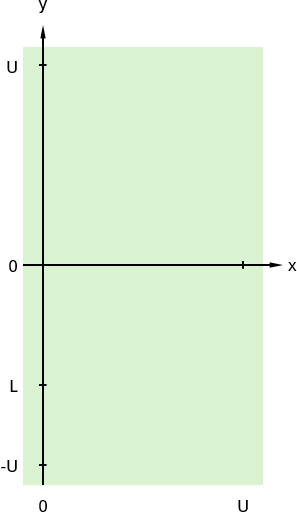
We start with the entire x-y plane as the feasible region. Part of the plane is shown in Figure 1, where the feasible region is shaded light green. We have also marked some points on the x and y axes that will be important as we add constraints.
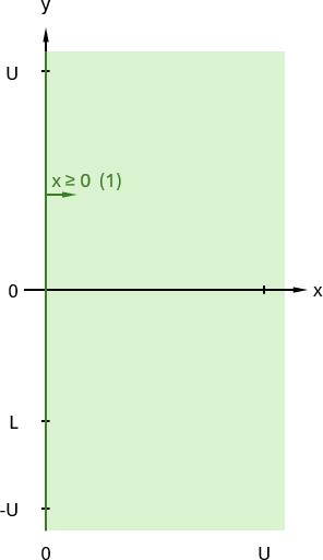
First, we apply the constraint \(x \ge 0\), as shown in Figure 2. This handles the requirement implicit in the question that \(x\) cannot be negative.
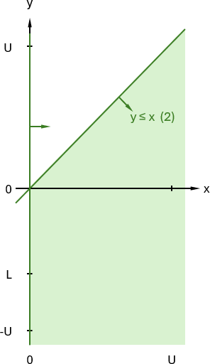
Then we apply the constraint \(y \le x\), as shown in Figure 3. This constraint, in conjunction with Equation (1), establishes a relationship between \(y\) and \(x\) when \(y \ge 0\).
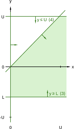
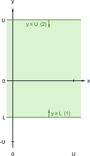
Although it isn't strictly required, and the proposed answer doesn't do this, we add bounds on the value of \(y\). These bounds reduce the conditions under which the model is unbounded. The model might have other constraints that perform a similar role, but here we have only the stated constraints. That is:
We assume that \(L\) is a negative number, as we want to allow \(y \le 0\). The new feasible region is shown in Figure 4.
Now we get to the part where the answer said "For some models". What this means is that we get the required behaviour if the objective function has an appropriate form.
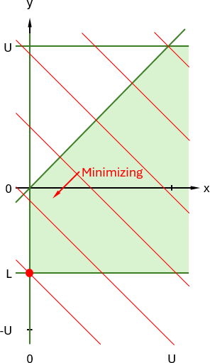
For example, if we are minimizing with the objective function contours shown in Figure 5, then we get an optimal solution that occurs at \(y = \text{L}\) (where \(\text{L}\) is negative), and \(x = 0\). This solution complies with the question's requirement that \(x = 0\) when \(y \le 0\).
But if we are maximizing this objective function, then the optimal solution would be somewhere in the positive \(x\) direction, where \(x \ge \text{U}\) (noting that the feasible region is open in the positive x direction, so the model may be unbounded). Without other constraints, that solution may not comply with the question's requirements as it allows \(x\) and \(y\) to have different values.
Conversely, if we are maximizing the objective function contours shown in Figure 6, then the optimal solution occurs at \(x = \text{U}\), and \(y = \text{U}\). This solution complies with the question's requirements.
But if we are minimizing this objective function, then the solution may not comply with the question's requirements.
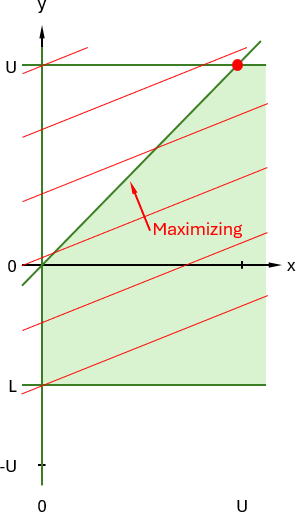
The exact form of the objective function is crucial to Formulation 1 working as intended. For example, we may have a situation where the model works correctly for a given objective function. But, due to a small change in the objective function parameters, the behaviour changes and the constraints no longer work as intended.
In summary, Formulation 1 works only if the objective function drives the solver to a solution that complies with the requirements. But not all objective functions work correctly. This formulation has the advantage of being linear and not requiring binary variables, but great care needs to be taken to ensure that the model does what we want.
Formulation 2
The second proposed formulation uses binary variables to choose between the two IF conditions. Using binary variables makes the model a mixed integer linear program, which might make it much more difficult to solve. But this method has the advantage of giving us more control over the solver's behaviour, so we don't need to rely on the form of the objective function, like we do in Formulation 1.
The answer on Stack Exchange includes a derivation, which is useful to understand for applying to similar situations. The resulting formulation, reordered for convenience of presentation here, is summarized in Figure 7. Note that we restart the constraint numbering, as this is a separate formulation.
The binary variable \(\delta\) is used to choose between the two IF statements in the question. We illustrate the behaviour of this formulation in the following figures.
Formulation 2, Case: \(\delta = 0\)
Firstly, we set \(\delta = 0\). We add each of the constraints, starting with the bounds on \(y\), as shown in Figure 8.
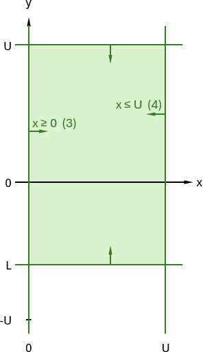
Next, we add the bounds on \(x\). Note that, since there is a requirement that \(x=y\) when \(y\) is positive, the upper bounds of \(x\) and \(y\) must be the same.
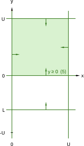
For this formulation, when \(\delta = 0\), Equation (5) \(\text{L} \times \delta \le y\) becomes \(y \ge 0\), as shown in Figure 10.
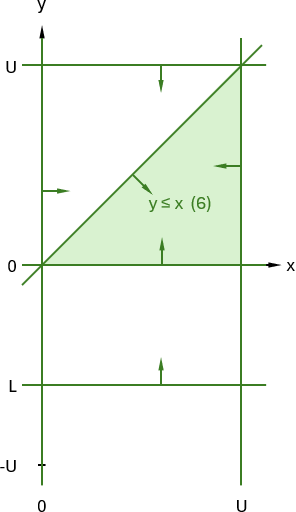
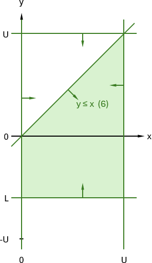
Next, we have Equation (6) \(y \le x\), like we have in Formulation 1. This constraint restricts the feasible region to the triangle shown in Figure 11.
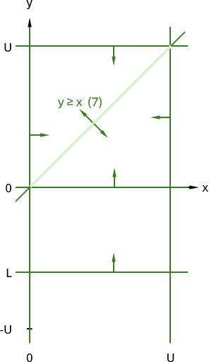
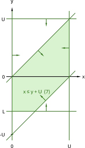
Finally, we apply Equation (7) \(x \le y + \text{U} \times \delta\). When \(\delta = 0\), this becomes \(x \le y\). As shown in Figure 12, this constraint reduces the feasible region to the line segment between (0, 0) and (U, U). In other words, \(\delta = 0\) creates the second IF condition: \(\text{if } y \gt 0, \text{then } x = y\).
Equation (8) for Formulation 2 is \(x \le \text{U} \times (1-\delta)\). When \(\delta = 0\), this becomes \(x \le \text{U}\). We already have this bound on \(x\), so we don't need to add it again.
Note that the question specifies \(\gt\), whereas we have \(\ge\). Constraints that are strictly "greater than" don't make sense in a linear program – though, as we'll see in the next section, enforcing the "equals" part doesn't change anything in this situation – because the IF statements coincide at the point (0, 0).
Formulation 2, Case: \(\delta = 1\)
Now we set \(\delta = 1\) and re-evaluate the constraints for Formulation 2.
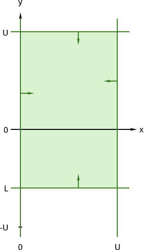
Equations (1) to (4) specify the same bounds on \(x\) and \(y\), as shown in Figure 13.
When \(\delta = 1\), Equation (5) \(\text{L} \times \delta \le y\) becomes \(\text{L} \le y\). This is the same as Equation (1), so we don't need to repeat it.
We add Equation (6) \(y \le x\), as shown in Figure 14.
When \(\delta = 1\), Equation (7) \(x \le y + \text{U} \times \delta\) becomes \(x \le y + \text{U}\), as shown in Figure 15.
Finally, we add Equation (8) \(x \le \text{U} \times (1-\delta)\), which becomes \(x \le 0\), as shown in Figure 16. The feasible region is reduced to the line segment between (0, 0) and (0, L). This feasible region creates the first IF condition: \(\text{if } y \le 0, \text{then } x = 0\).
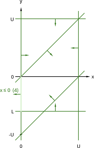
Figures 12 and 16 illustrate how, depending on the value of \(\delta\), Formulation 2's constraints produce the behaviour required in the question's IF statements.
But there's a problem
In our diagrams, we've illustrated the situation where \(L\) is a negative number and \(U\) is a positive number. The constraints correctly account for the assumed signs of the bounds, so that's OK.
We've also assumed that the absolute value of \(L\) is less than the absolute value of \(U\). In Figure 16 above, Equation (7) passes through (0, -U). Since \(-U\) is below \(L\), Equation (7) doesn't affect the feasible region, as intended.
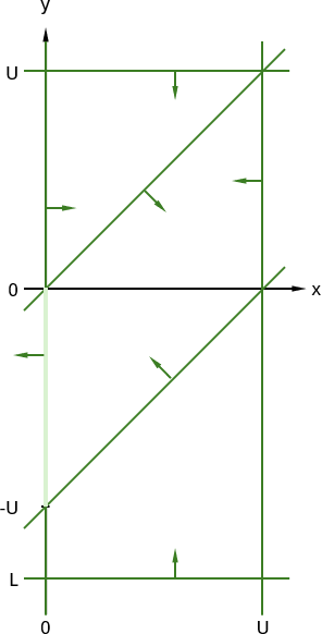
But what if the absolute value of \(L\) is greater than the absolute value of \(U\)? This situation is shown in Figure 17. Equation (7) is binding, limiting the feasible region to the range (0, 0) to (0, -U). The vertical range is supposed to be within the bounds \(L \le y \le U\), but it isn't. So, this formulation is incorrect.
A comment on the Stack Exchange question points out the error in Equation (7), suggesting that the constraint could be strengthened by changing it from \(x \le y + \text{U} \times \delta\) to \(x \le y - \text{L} \times \delta\).
Strengthening, or "tightening", constraints is an important concept in math programming. Tighter constraints reduce the size of the feasible region, usually producing a faster solve time.
But in the case where \(-U\) is smaller than \(L\), Equation (7) is overly tight – reducing the size of the feasible region beyond what is intended. Therefore, the proposed strengthening doesn't just make the formulation tighter, it corrects a subtle error in Formulation 2.
Formulation 3
Another formulation is proposed in the Stack Exchange answers. It starts with the observation that the required IF statements are equivalent to \(x = max(y, 0)\). The answer then derives constraints that we summarize in Figure 18.
Formulation 3 is very similar to Formulation 2, though the differences are important: Equation (5) from Formulation 2 is not required, and Equation (7) differs from Formulation 2.
Formulation 3, Case: \(\delta = 0\)
For \(\delta = 0\), Formulation 3 is the same as Formulation 2. The constraints are shown in Figure 19, which is the same as Figure 12. The feasible region is the line segment from (0, 0) to (U, U), representing the IF statement that requires \(x = y\) when \(y\) is positive.
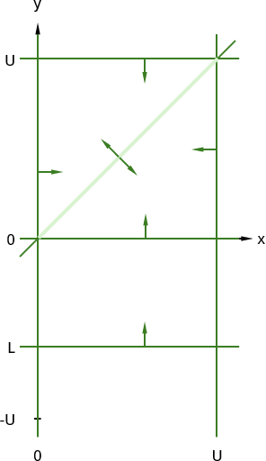
Formulation 3, Case: \(\delta = 1\)
For \(\delta = 1\), Formulation 3 is initially the same as Formulation 2. That is, the bounds on \(x\) and \(y\) are identical, and we have Equation (6) \(y \le x\), as shown in Figure 20.
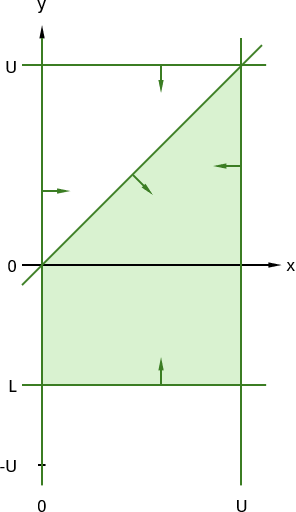
Equation (7) differs from the equivalent constraint in Formulation 2, producing the feasible region shown in Figure 21. Importantly, the constraint goes through the point (0, L) rather than (0, -U).
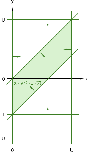
Consequently, when we apply Equation (8) in Figure 22, the feasible region is the line segment from (0, 0) to (0, L), as intended.
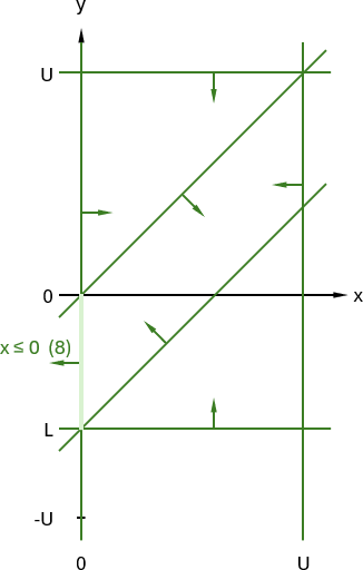
In the case where \(L\) is below \(-U\), Formulation 2 produces an incorrect feasible region (shown in Figure 17 above). But, as shown in Figure 23, Formulation 3 produces the correct feasible region of a line segment between (0, 0) and (0, L).
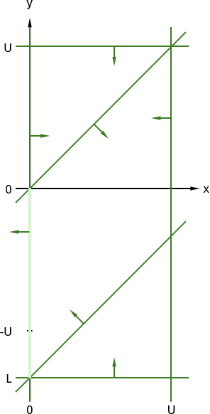
Formulation 3's constraints implement the question's IF statements. Importantly, note that all of the constraints are applied all the time. The \(\delta\) binary variable acts as a switch, changing the constraints in a way that mimics the behaviour defined by the two IF statements.
Formulation 4
Formulation 3 correctly produces the behaviour required by the original question. Therefore, the question has been answered.
However, it might be useful to add one more formulation. A couple of the Stack Exchange answers include derivations of their constraints. This is very helpful for understanding how to answer similar questions. In that spirit, we derive a formulation for the original question from a more general case.
We start with a formulation for the constraint \(x = max(y, z)\). This formulation is from Professor Rubin's blog Max and Min Functions in a MIP. Note that we've translated the notation to be consistent with the formulations above.
The formulation for the constraint \(x = max(y, z)\) is shown in Figure 24.
Recall that Formulation 3 noted that the required IF statements are equivalent to \(x = max(y, 0)\). This is a special case of \(x = max(y, z)\), where \(z = 0\). Therefore, we can derive that special case by setting \(z = 0\) and simplifying the formulation in Figure 24. The result is shown in Figure 25.
Professor Prubin notes that Equations (5) and (6) are sometimes sufficient. That is essentially what Formulation 1 does.
The first parts of Formulation 4 are very similar to Formulation 3. That is, as shown in Figure 26, we have lower and upper bounds on \(y\), a lower bound on \(x\), and the constraint \(x \ge y\). Note that, at this stage, we don't have an upper bound on \(x\).
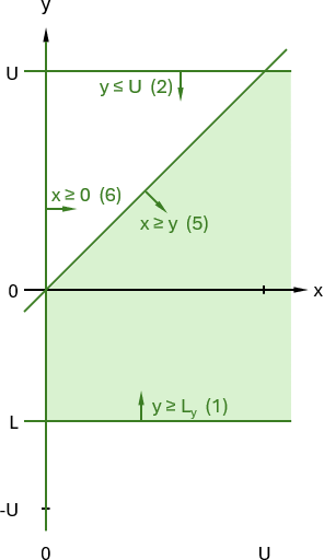
Equations (7) and (8) include the binary variable \(\delta\). When we evaluate those constraints for either \(\delta = 0\) or \(\delta = 1\), the result is as shown in Figure 27.
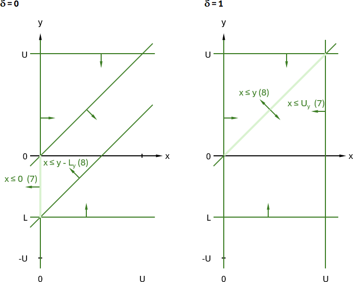
Like for Formulations 2 and 3, the \(\delta\) binary variable acts as a switch between the two IF statements. When \(\delta = 0\), the feasible region is the line segment from (0, 0) to (0, L). When \(\delta = 1\), the feasible region is the line segment from (0, 0) to (U, U). This is what was required in the original question, so Formulation 4 also works correctly.
Note an important difference between Formulation 3 and Formulation 4: the meaning of \(\delta\) is reversed. This is reassuring, because the meaning of \(\delta\) is arbitrary. There is no specific reason why \(\delta = 0\) must represent one or other of the IF statements. In Formulation 4, we just happen to use the opposite meaning to that used in Formulation 3. The constraints perform the same role, so either definition works correctly – as it should for an arbitrary definition.
Conclusion
In this article, we illustrate some answers to a common class of linear programming questions: How can I represent IF statements in an LP?
The specific question we examine is from Operations Research Stack Exchange, where three different answers are suggested. Formulation 1 works in a special case, Formulation 2 works in most situations but it has a subtle error, and Formulation 3 is correct. Here we provide a fourth answer, deriving a formulation from a more general situation.
Formulation 1 shows that we need to be aware of the conditions in which a specific formulation is valid, or not. Formulation 2 shows that we need to carefully verify that our formulation is correct in all cases.
Translating requirements, such as IF statements, into a form that a solver can work with is an essential skill in optimization modelling. A linear program cannot implement IF statements but, with an appropriate transformation, we can formulate constraints that mimic the behaviour we want. Being able to derive and apply such constraints opens a whole new world for a math programming modeller.
If you would like to know more about this model, or you want help with your own models, then please contact us.


