23 July 2024

We continue our exploration of methods to solve our device rack positioning problem. The methods are:
- Model 1. Enumerate all possible position orders.
- Model 2. Search randomly for a specified time.
- Model 3. Local search around random starting positions.
- Model 4. Constraint programming using OR-Tools.
- Model 5. Mixed integer linear programming using Pyomo.
The previous article describes Model 1, which uses enumeration of all possible permutations. That method works well for a small number of devices, up to about 12. But it fails to find good solutions for larger data sets because it takes too long to run – up to tens of billions of years, for the larger cases.
In this article, we develop Model 2, which tries a parallel random search method. The idea is to randomly generate possible solutions for a specified time, reporting the best solution we find. This method has an advantage over enumeration: it samples from all parts of the solution space, unlike Model's 1 enumeration method which is limited by run time to a specific part of the solution space. But will Model 2 perform better than Model 1?
Download the models
The models described in this series of articles are built in Python.
The files are available on GitHub.
Situation
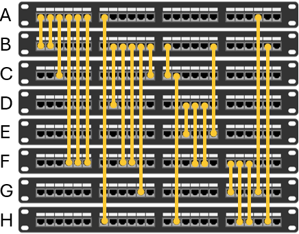
The situation is described fully in the previous article. Briefly, we have network devices in a rack. We need to use cables to connect each device to one or more other devices in the rack, arranged like in Figure 1. The question is, in what order should we position the devices to minimize the total cable length?
Model 2 design
Model 2 generates and evaluates random device orders until it has completed a specified number of iterations or it runs out of time. Since each iteration is independent of other iterations, we can evaluate them in parallel – so we design the model to use all the PC's CPU cores/threads, to make the search faster. The model prints a progress report of the best objective function value found so far. At the end it reports the best solution found.
Model 2 implementation
Data structure
Model 2 uses the same input data structure used by Model 1.
Differences from Model 1
We start with the code for Model 1 and make two substantial changes to produce Model 2:
- Instead of systematically enumerating device orders, at each iteration Model 2 randomly shuffles the device order using
random.shuffle(order). Because we shuffle the device order list "in place" (i.e., within the existing data structure), when we note a new best solution, we need to perform a deep copy of the order list. A shallow copy would return an incorrect result after the order list is shuffled in the next iteration, because a shallow copy would point to the order list object that we're shuffling. A deep copy creates a new object, so it retains the best solution when the order list is shuffled. For a description of shallow versus deep copy, see Shallow vs deep copy in Python. - The device orders are divided into "chunks" and assigned to each of the CPU's cores/threads to run in parallel using the multiprocessing library. Since the orders are independent, the only communication we need between iterations is for reporting the current best solution found. This is achieved via a shared dictionary, which is locked by each process while updating. To ensure efficency, we update progress only every 5 seconds.
The code for processing each chuck is shown in Figure 2. This code is run by each process in parallel.
def cable_layout_chunk(start, end, cable_struct, num_devices, start_time, shared_dict, max_time):    # Each processor's chunk of the solution space
    local_min_length = float('inf')    # Best length found by this process
    local_best_case = []    # Best case found by this process
    order = list(range(num_devices))
    last_update = time.time()

    for done in range(start, end):
        random.shuffle(order)    # Create a random device order
        length = calculate_total_length(order, cable_struct)

        if length < local_min_length:
            local_best_case = copy.deepcopy(order)    # Need deep copy as order is shuffled in place
            local_min_length = length

        current_time = time.time()
        if current_time - last_update >= UPDATE_INTERVAL:    # At some interval, co-ordinate with other processes to note progress. Multiple processes may print an update
            with shared_dict['lock']:
                pct_done = (done - start) / (end - start)
                if local_min_length < shared_dict['min_length']:    # Update best solution found so far (note <)
                    shared_dict['new_best'] = True
                    shared_dict['min_length'] = local_min_length
                    shared_dict['best_case'] = local_best_case
                    shared_dict['pct_done'] = pct_done
                if (local_min_length <= shared_dict['min_length']) and (pct_done >= shared_dict['last_pct_done']):    # Print progress, even if no improvement (note <=)
                    elapsed_time = current_time - start_time
                    shared_dict['last_pct_done'] = pct_done
                    print_progress(elapsed_time, local_min_length, pct_done, shared_dict['new_best'])
                    shared_dict['new_best'] = False
            last_update += UPDATE_INTERVAL    # Defer updating until next regular update time

        if (current_time - start_time) >= max_time:    # Stop search if reached maximum overall run time
            break
    return local_min_length, local_best_case, done - start + 1
With a little help from my friend, Claude
We've used the multiprocessing library previously, for example in the article 10 times faster, running cases in parallel. For this model, we wanted to take a different approach, using parts of the multiprocessing library that we weren't familiar with.
Since getting the syntax correct can be quite tricky, we enlisted the Claude AI to help us write the parallel part of the code. Our previous experiences with using AI as a coding assistant have been disappointing, with the AI being more hinderance than help. But our most recent attempt was six months ago, while AI is developing rapidly. This time, our experience was better in that Claude was helpful, though still a bit frustrating.
The goal was for Claude to modify our initial single-threaded program to be multi-threaded. This was successful, but it took several attempts to get code that uses the CPU cores/threads fully. Claude's first attempt at parallel code was slower than our single-threaded code because Claude included a lot of unnecessary thread-blocking communication between the processes. With some persuasion, Claude simplified the code and made it much faster.
Of greater concern is that Claude introduced errors and subtle bugs. For example:
- Claude sometimes writes invalid code, like using properties that don't exist or code that is inconsistent with another part of the code. When we paste the error message and ask for a correction, Claude is usually able to correct the code at the next attempt while apologizing for the "oversight".
- Claude kept removing the deep copy, saying it is slow and unnecessary. Deep copying can be slow but, as explained above, it is necessary in this situation because a standard shallow copy may return an incorrect result. If we were not aware of the need to do a deep copy, then this bug might have been difficult to identify.
- Claude repeatedly changed our line
last_update += UPDATE_INTERVALtolast_update = current_time. Claude's version is a more common approach, which is probably why it insisted on making the change. But, because there is significant code between whencurrent_timeis defined and when it is used in that line, Claude's change causes the update time to slowly creep out of step with the intended 5-second interval. Attempts to convince Claude to keep our line of code were unsuccessful. - Finally, Claude did not consistently use the shared dictionary that it created, leading to an occasional subtle error in printing the best solution.
Despite these issues, we found Claude to be helpful for creating the general structure and detailed syntax to make our code run in parallel. That saved us a lot of time. But Claude's code is of variable quality, so it must be carefully reviewed and tested. We needed to invest time to understand, and sometimes modify, Claude's code to fix bugs and ensure that it does exactly what we want.
Overall, our experience with this model suggests that coding using an AI can be useful, but only as an assistant for small and specific tasks, rather than for writing substantial pieces of code. We liken the process of using Claude AI to working with a knowledgeable but over-confident junior analyst – useful, but Claude can't be trusted to work independently. Yet.
Model 2 results
Model output
Figure 3 shows an example of the model output when running the data for 12 devices with a time limit of 60 seconds. In this relatively small example, 60 seconds is long enough to run more than 300 million iterations – which equates to most of the 479 million possible permutations. The random process will likely evaluate duplicate cases, so the percentage done is not entirely accurate. After about 25 seconds, Model 2 finds the optimal solution of 60 decimetres (though this model doesn't know that the solution is optimal).
Model 2: Cable length management, random sample in parallel

     Time    %done     Best
---------------------------
        5    5.87%     62 *
        5    5.91%     61 *
        5    6.10%     61
        5    6.19%     61
       10   12.24%     61
       10   12.32%     61
       15   17.05%     61
       15   17.38%     61
       15   18.30%     61
       15   18.31%     61
       20   22.01%     61
       25   25.35%     60 *
       30   30.28%     60
       35   35.25%     60
       40   40.17%     60
       40   46.10%     60
       45   51.06%     60
       50   56.01%     60
       55   62.42%     60

Devices: 12
Minimum length: 60
Best case: ['K', 'L', 'C', 'H', 'B', 'A', 'F', 'D', 'G', 'I', 'E', 'J']
Done 315,218,936 of 479,001,600 cases (65.81%)
Time: 60.05 seconds
Rate: 5,249,557 cases per second
Comparison between methods
In Figure 4 we compare the best solutions found by Model 2 with the best solutions found by Model 1. Both models ran for up to 1 hour for each data set (number of devices).
Model 2 finds optimal solutions for 8 to 12 devices within the 1 hour limit. We know that those solutions are optimal because Model 1 proved them to be optimal. For more devices, both Model 1 and Model 2 stop at the 1 hour time limit, so we don't know if those solutions are optimal. Nonetheless, for 13 to 24 devices, Model 2's random search solutions are all better than those found by enumeration in Model 1. For the larger data sets, Model 2's solutions are around 50% better given the same run time.
Note that Model 2's solution for 19 devices is lower than its solution for 18 devices. Since the length must increase as we add devices, this tells us that a better solution for 18 devices must exist. It also suggests that better solutions for 20+ devices are likely to exist.
Why is random search better than enumeration?
It all depends on where you look
In this situation, the random search method of Model 2 is substantially better than the enumeration method of Model 1. Why is that?
We can get a hint by looking at the first dozen iterations evaluated by Model 1 and Model 2, for 8 devices, as shown in Figure 5.
The enumeration process in Model 1 starts with the devices in alphabetical order and then explores variations in the order from there. All the iterations are very similar, being in the same neighbourhood of the solution space, and so the cable lengths are fairly similar. The best iteration in this sample has a length of 69 decimetres.
The random search process in Model 2 produces a much more varied range of device orders, sampling orders from throughout the solution space. The best iteration in this sample has a length of 48 decimetres – close to the optimal solution of 46 decimetres.
Good solutions are extremely rare
For the data set with 8 devices, we can plot the distribution of objective function values for all possible solutions, as shown in Figure 6. With 8 devices, there are 8! = 40,320 possible permutations of the device order. The distribution of total cable lengths is roughly normally distributed, ranging from 46 to 97 with an average of 69. It also has an interesting feature of alternating spikes. The optimal solutions have a length of 46 decimetres, which occurs 6 times out of the 40,320 possibilities – so infrequent that it is not visible on the chart.
If we have more devices, then the distribution has a similar shape but with many more cases. The number of cases that are at or close to optimal becomes proportionately smaller and so good solutions are harder to find. As the number of cases increases, the likelihood that a given solution is close to optimal becomes vanishingly small.
Nonetheless, the process of picking random orders gives Model 2 a much better chance of picking at least a good solution – which it does.
How much do we gain from parallelism?
A secondary reason why the random search method produces better solutions than the enumeration method is that the search is conducted in parallel while the enumeration is single-threaded. However, running in parallel doesn't make as much difference as we might hope.
If we restrict the search to a single thread then, for the 24 device data set, Model 2 evaluates about 200,000 cases per second – slightly slower than Model 1 because of the shuffling process and the multiprocessing library's overhead. Using all our PC's 20 cores / 28 threads in parallel, Model 2 evaluates over 3,000,000 cases per second – about 15 times faster. For the smaller 12 device data, the parallel method evaluates over 5,000,000 cases per second – also about 15 times faster than running single-threaded.
But the best solutions from the parallel version are only slightly better than those found by running single-threaded. For example, running single-threaded for one hour, Model 2's best solution for 24 devices has a length of 190 decimetres. Running in parallel for the same time limit produced a best solution of 178 decimetres. That's materially better, but not by a large margin (though both solutions are substantially better than the solution found by enumeration).
We achieve only modest gains from evaluating 15 times as many cases simply because good solutions are uncommon and become extremely rare as we approach the left tail of the distrbution – as shown in Figure 6. The vast majority of the solutions Model 2 finds are in the bulk of the distribution, while what we want is in the extreme left tail of the distribution. Evaluating more cases improves the odds of finding good solutions, but for the larger data sets the number of possible cases is so enormous that close to optimal solutions are extremely unlikely to be found by searching randomly.
Next steps
By using a random search method, we've been able to significantly improve the solutions for the larger data sets. But, because the solutions are not proven optimal, perhaps we can improve the solutions further?
So, in the next article, we refine our random search method by adding a local search process. The idea is to look around the solution space of good solutions, to see if there are better solutions nearby.
Conclusion
In this article, we use a random search method to find good solutions to our problem of positioning devices in a rack.
Model 2's parallel random search strategy works surprisingly well in this situation. It is much better than Model 1's enumeration method when the solution space is too large to enumerate fully.
Even though we have better solutions for 13+ devices, none of those solutions have been proven optimal. It might be possible to do even better by using a slightly more sophisticated method. Therefore, in the next article, we add a local search method to our model.
If you would like to know more about this model, or you want help with your own models, then please contact us.

